YOLOv7: Trainable Bag-of-Freebies

YOLOv7, được phát hành vào tháng 7 năm 2022, là một bước tiến quan trọng trong lĩnh vực phát hiện đối tượng thời gian thực vào thời điểm ra mắt. Model này đạt 56.8% AP trên GPU V100, thiết lập các benchmark mới khi được giới thiệu. YOLOv7 vượt trội hơn các trình phát hiện đối tượng đương thời như YOLOR, YOLOX, Scaled-YOLOv4 và YOLOv5 về tốc độ và accuracy. Model được huấn luyện từ đầu trên bộ dữ liệu MS COCO mà không sử dụng bất kỳ bộ dữ liệu nào khác hoặc trọng số được huấn luyện trước (pretrained weights). Mã nguồn của YOLOv7 có sẵn trên GitHub. Lưu ý rằng các model mới hơn như YOLO11 và YOLO26 đã đạt được độ chính xác cao hơn với hiệu suất được cải thiện kể từ đó.

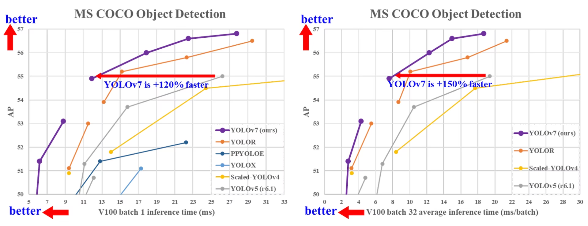
So sánh các trình phát hiện đối tượng SOTA

Từ kết quả trong bảng so sánh YOLO, chúng ta biết rằng phương pháp được đề xuất có sự cân bằng tốt nhất về tốc độ-độ chính xác một cách toàn diện. Nếu so sánh YOLOv7-tiny-SiLU với YOLOv5-N (r6.1), phương pháp của chúng tôi nhanh hơn 127 fps và chính xác hơn 10.7% về AP. Ngoài ra, YOLOv7 có 51.4% AP ở tốc độ khung hình 161 fps, trong khi PPYOLOE-L với cùng AP chỉ đạt tốc độ khung hình 78 fps. Về mức độ sử dụng tham số, YOLOv7 thấp hơn 41% so với PPYOLOE-L.

Nếu so sánh YOLOv7-X với tốc độ suy luận 114 fps với YOLOv5-L (r6.1) với tốc độ suy luận 99 fps, YOLOv7-X có thể cải thiện AP thêm 3.9%. Nếu YOLOv7-X được so sánh với YOLOv5-X (r6.1) ở quy mô tương tự, tốc độ suy luận của YOLOv7-X nhanh hơn 31 fps. Ngoài ra, về mặt số lượng tham số và tính toán, YOLOv7-X giảm 22% số lượng tham số và 8% khối lượng tính toán so với YOLOv5-X (r6.1), nhưng cải thiện AP thêm 2.2% (Nguồn).

Tổng quan

Phát hiện đối tượng thời gian thực là một thành phần quan trọng trong nhiều computer vision hệ thống, bao gồm theo dõi đa đối tượng, lái xe tự động, robot học, và và phân tích hình ảnh y tế. Trong những năm gần đây, sự phát triển của công nghệ phát hiện đối tượng thời gian thực tập trung vào việc thiết kế các kiến trúc hiệu quả và cải thiện tốc độ suy luận trên nhiều CPU, GPU và NPU khác nhau. YOLOv7 hỗ trợ cả thiết bị GPU di động và GPU, từ biên (edge) cho đến đám mây (cloud).

Không giống như các trình phát hiện đối tượng thời gian thực truyền thống tập trung vào tối ưu hóa kiến trúc, YOLOv7 giới thiệu trọng tâm vào tối ưu hóa quy trình huấn luyện. Điều này bao gồm các module và phương pháp tối ưu hóa được thiết kế để cải thiện độ chính xác khi phát hiện đối tượng mà không làm tăng chi phí suy luận, một khái niệm được gọi là "trainable bag-of-freebies".

Các tính năng chính

YOLOv7 giới thiệu một số tính năng chính:

1. Tái tham số hóa mô hình (Model Re-parameterization): YOLOv7 đề xuất một mô hình tái tham số hóa có kế hoạch, đây là một chiến lược áp dụng cho các lớp trong các mạng khác nhau với khái niệm đường dẫn truyền gradient.

2. Gán nhãn động (Dynamic Label Assignment): Việc huấn luyện mô hình với nhiều lớp đầu ra tạo ra một vấn đề mới: "Làm thế nào để gán các mục tiêu động cho đầu ra của các nhánh khác nhau?" Để giải quyết vấn đề này, YOLOv7 giới thiệu một phương pháp gán nhãn mới gọi là gán nhãn có hướng dẫn từ thô đến tinh (coarse-to-fine lead guided label assignment).

3. Mở rộng và mở rộng hợp chất (Extended and Compound Scaling): YOLOv7 đề xuất các phương pháp "extend" (mở rộng) và "compound scaling" (mở rộng hợp chất) cho bộ phát hiện đối tượng thời gian thực, cho phép tận dụng hiệu quả các tham số và tính toán.

4. Hiệu quả: Phương pháp do YOLOv7 đề xuất có thể giảm hiệu quả khoảng 40% tham số và 50% tính toán của các trình phát hiện đối tượng thời gian thực hiện đại, đồng thời có tốc độ suy luận nhanh hơn và độ chính xác phát hiện cao hơn.

Ví dụ sử dụng

Ultralytics không công bố yolov7.pt trọng số tiền huấn luyện hoặc ultralytics/cfg/models/v7/ các file YAML, và việc huấn luyện cũng như suy luận PyTorch gốc cho YOLOv7 không được hỗ trợ bởi gói Python của Ultralytics. Tuy nhiên, bạn có thể đưa checkpoint YOLOv7 được huấn luyện trong upstream YOLOv7 repository vào Ultralytics bằng cách xuất nó sang ONNX hoặc TensorRT, như được hiển thị bên dưới.

Xuất ONNX

Để sử dụng mô hình ONNX của YOLOv7 với Ultralytics:

1. (Tùy chọn) Cài đặt Ultralytics và xuất một mô hình ONNX để các phụ thuộc cần thiết được tự động cài đặt:

   pip install ultralytics
   yolo export model=yolo26n.pt format=onnx

2. Xuất mô hình YOLOv7 mong muốn bằng cách sử dụng bộ xuất trong repo YOLOv7:

   git clone https://github.com/WongKinYiu/yolov7
   cd yolov7
   python export.py --weights yolov7-tiny.pt --grid --end2end --simplify --topk-all 100 --iou-thres 0.65 --conf-thres 0.35 --img-size 640 640 --max-wh 640

3. Sửa đổi đồ thị mô hình ONNX để tương thích với Ultralytics bằng cách sử dụng script sau:

   import numpy as np
   import onnx
   from onnx import helper, numpy_helper
   
   # Load the ONNX model
   model_path = "yolov7/yolov7-tiny.onnx"  # Replace with your model path
   model = onnx.load(model_path)
   graph = model.graph
   
   # Fix input shape to batch size 1
   input_shape = graph.input[0].type.tensor_type.shape
   input_shape.dim[0].dim_value = 1
   
   # Define the output of the original model
   original_output_name = graph.output[0].name
   
   # Create slicing nodes
   sliced_output_name = f"{original_output_name}_sliced"
   
   # Define initializers for slicing (remove the first value)
   start = numpy_helper.from_array(np.array([1], dtype=np.int64), name="slice_start")
   end = numpy_helper.from_array(np.array([7], dtype=np.int64), name="slice_end")
   axes = numpy_helper.from_array(np.array([1], dtype=np.int64), name="slice_axes")
   steps = numpy_helper.from_array(np.array([1], dtype=np.int64), name="slice_steps")
   
   graph.initializer.extend([start, end, axes, steps])
   
   slice_node = helper.make_node(
       "Slice",
       inputs=[original_output_name, "slice_start", "slice_end", "slice_axes", "slice_steps"],
       outputs=[sliced_output_name],
       name="SliceNode",
   )
   graph.node.append(slice_node)
   
   # Define segment slicing
   seg1_start = numpy_helper.from_array(np.array([0], dtype=np.int64), name="seg1_start")
   seg1_end = numpy_helper.from_array(np.array([4], dtype=np.int64), name="seg1_end")
   seg2_start = numpy_helper.from_array(np.array([4], dtype=np.int64), name="seg2_start")
   seg2_end = numpy_helper.from_array(np.array([5], dtype=np.int64), name="seg2_end")
   seg3_start = numpy_helper.from_array(np.array([5], dtype=np.int64), name="seg3_start")
   seg3_end = numpy_helper.from_array(np.array([6], dtype=np.int64), name="seg3_end")
   
   graph.initializer.extend([seg1_start, seg1_end, seg2_start, seg2_end, seg3_start, seg3_end])
   
   # Create intermediate tensors for segments
   segment_1_name = f"{sliced_output_name}_segment1"
   segment_2_name = f"{sliced_output_name}_segment2"
   segment_3_name = f"{sliced_output_name}_segment3"
   
   # Add segment slicing nodes
   graph.node.extend(
       [
           helper.make_node(
               "Slice",
               inputs=[sliced_output_name, "seg1_start", "seg1_end", "slice_axes", "slice_steps"],
               outputs=[segment_1_name],
               name="SliceSegment1",
           ),
           helper.make_node(
               "Slice",
               inputs=[sliced_output_name, "seg2_start", "seg2_end", "slice_axes", "slice_steps"],
               outputs=[segment_2_name],
               name="SliceSegment2",
           ),
           helper.make_node(
               "Slice",
               inputs=[sliced_output_name, "seg3_start", "seg3_end", "slice_axes", "slice_steps"],
               outputs=[segment_3_name],
               name="SliceSegment3",
           ),
       ]
   )
   
   # Concatenate the segments
   concat_output_name = f"{sliced_output_name}_concat"
   concat_node = helper.make_node(
       "Concat",
       inputs=[segment_1_name, segment_3_name, segment_2_name],
       outputs=[concat_output_name],
       axis=1,
       name="ConcatSwapped",
   )
   graph.node.append(concat_node)
   
   # Reshape to [1, -1, 6]
   reshape_shape = numpy_helper.from_array(np.array([1, -1, 6], dtype=np.int64), name="reshape_shape")
   graph.initializer.append(reshape_shape)
   
   final_output_name = f"{concat_output_name}_batched"
   reshape_node = helper.make_node(
       "Reshape",
       inputs=[concat_output_name, "reshape_shape"],
       outputs=[final_output_name],
       name="AddBatchDimension",
   )
   graph.node.append(reshape_node)
   
   # Get the shape of the reshaped tensor
   shape_node_name = f"{final_output_name}_shape"
   shape_node = helper.make_node(
       "Shape",
       inputs=[final_output_name],
       outputs=[shape_node_name],
       name="GetShapeDim",
   )
   graph.node.append(shape_node)
   
   # Extract the second dimension
   dim_1_index = numpy_helper.from_array(np.array([1], dtype=np.int64), name="dim_1_index")
   graph.initializer.append(dim_1_index)
   
   second_dim_name = f"{final_output_name}_dim1"
   gather_node = helper.make_node(
       "Gather",
       inputs=[shape_node_name, "dim_1_index"],
       outputs=[second_dim_name],
       name="GatherSecondDim",
   )
   graph.node.append(gather_node)
   
   # Subtract from 100 to determine how many values to pad
   target_size = numpy_helper.from_array(np.array([100], dtype=np.int64), name="target_size")
   graph.initializer.append(target_size)
   
   pad_size_name = f"{second_dim_name}_padsize"
   sub_node = helper.make_node(
       "Sub",
       inputs=["target_size", second_dim_name],
       outputs=[pad_size_name],
       name="CalculatePadSize",
   )
   graph.node.append(sub_node)
   
   # Build the [2, 3] pad array:
   # 1st row -> [0, 0, 0] (no padding at the start of any dim)
   # 2nd row -> [0, pad_size, 0] (pad only at the end of the second dim)
   pad_starts = numpy_helper.from_array(np.array([0, 0, 0], dtype=np.int64), name="pad_starts")
   graph.initializer.append(pad_starts)
   
   zero_scalar = numpy_helper.from_array(np.array([0], dtype=np.int64), name="zero_scalar")
   graph.initializer.append(zero_scalar)
   
   pad_ends_name = "pad_ends"
   concat_pad_ends_node = helper.make_node(
       "Concat",
       inputs=["zero_scalar", pad_size_name, "zero_scalar"],
       outputs=[pad_ends_name],
       axis=0,
       name="ConcatPadEnds",
   )
   graph.node.append(concat_pad_ends_node)
   
   pad_values_name = "pad_values"
   concat_pad_node = helper.make_node(
       "Concat",
       inputs=["pad_starts", pad_ends_name],
       outputs=[pad_values_name],
       axis=0,
       name="ConcatPadStartsEnds",
   )
   graph.node.append(concat_pad_node)
   
   # Create Pad operator to pad with zeros
   pad_output_name = f"{final_output_name}_padded"
   pad_constant_value = numpy_helper.from_array(
       np.array([0.0], dtype=np.float32),
       name="pad_constant_value",
   )
   graph.initializer.append(pad_constant_value)
   
   pad_node = helper.make_node(
       "Pad",
       inputs=[final_output_name, pad_values_name, "pad_constant_value"],
       outputs=[pad_output_name],
       mode="constant",
       name="PadToFixedSize",
   )
   graph.node.append(pad_node)
   
   # Update the graph's final output to [1, 100, 6]
   new_output_type = onnx.helper.make_tensor_type_proto(
       elem_type=graph.output[0].type.tensor_type.elem_type, shape=[1, 100, 6]
   )
   new_output = onnx.helper.make_value_info(name=pad_output_name, type_proto=new_output_type)
   
   # Replace the old output with the new one
   graph.output.pop()
   graph.output.extend([new_output])
   
   # Save the modified model
   onnx.save(model, "yolov7-ultralytics.onnx")

4. Sau đó, bạn có thể tải mô hình ONNX đã sửa đổi và chạy suy luận với nó trong Ultralytics như bình thường:

   from ultralytics import ASSETS, YOLO
   
   model = YOLO("yolov7-ultralytics.onnx", task="detect")
   
   results = model(ASSETS / "bus.jpg")

Xuất TensorRT

1. Thực hiện theo các bước 1-2 trong Xuất ONNX .

2. Cài đặt gói TensorRT Python:

   pip install tensorrt

3. Chạy script sau để chuyển đổi mô hình ONNX đã sửa đổi sang engine TensorRT:

   from ultralytics.utils.export import export_engine
   
   export_engine("yolov7-ultralytics.onnx", half=True)

4. Tải và chạy mô hình trong Ultralytics:

   from ultralytics import ASSETS, YOLO
   
   model = YOLO("yolov7-ultralytics.engine", task="detect")
   
   results = model(ASSETS / "bus.jpg")

Trích dẫn và Ghi nhận

Chúng tôi muốn ghi nhận các tác giả của YOLOv7 vì những đóng góp quan trọng của họ trong lĩnh vực phát hiện đối tượng thời gian thực:

@article{wang2022yolov7,
  title={YOLOv7: Trainable bag-of-freebies sets new state-of-the-art for real-time object detectors},
  author={Wang, Chien-Yao and Bochkovskiy, Alexey and Liao, Hong-Yuan Mark},
  journal={arXiv preprint arXiv:2207.02696},
  year={2022}
}

Bài báo YOLOv7 gốc có thể được tìm thấy trên arXiv. Các tác giả đã công bố công trình của họ một cách công khai, và codebase có thể được truy cập trên GitHubGitHub. Chúng tôi đánh giá cao những nỗ lực của họ trong việc thúc đẩy lĩnh vực này và giúp cộng đồng rộng lớn hơn có thể tiếp cận công trình của họ.

FAQ

YOLOv7 là gì và tại sao nó được coi là một bước đột phá trong object detection?

phát hiện đối tượng thời gian thực? YOLOv7, được phát hành vào tháng 7 năm 2022, là một mô hình phát hiện đối tượng thời gian thực quan trọng đạt được tốc độ và độ chính xác tuyệt vời tại thời điểm phát hành. Nó vượt qua các mô hình đương thời như YOLOX, YOLOv5 và PPYOLOE cả về việc sử dụng tham số và tốc độ suy luận. Các tính năng nổi bật của YOLOv7 bao gồm tái tham số hóa mô hình và gán nhãn động, giúp tối ưu hóa hiệu suất mà không làm tăng chi phí suy luận. Để biết thêm chi tiết kỹ thuật về kiến trúc và các chỉ số so sánh với các trình phát hiện đối tượng hiện đại khác, hãy tham khảo bài báo YOLOv7.

YOLOv7 cải thiện như thế nào so với các mô hình YOLO trước đây như YOLOv4 và YOLOv5?

YOLOv7 giới thiệu một số đổi mới, bao gồm tái tham số hóa mô hình và gán nhãn động, giúp nâng cao quy trình huấn luyện và cải thiện độ chính xác khi suy luận. So với YOLOv5, YOLOv7 tăng đáng kể tốc độ và độ chính xác. Ví dụ, YOLOv7-X cải thiện độ chính xác thêm 2.2% và giảm 22% tham số so với YOLOv5-X. So sánh chi tiết có thể được tìm thấy trong bảng hiệu suất so sánh YOLOv7 với các trình phát hiện đối tượng SOTA.

Tôi có thể sử dụng YOLOv7 với các công cụ và nền tảng của Ultralytics không?

Hiện tại, Ultralytics chỉ hỗ trợ suy luận YOLOv7 định dạng ONNX và TensorRT. Để chạy phiên bản YOLOv7 đã xuất sang ONNX và TensorRT với Ultralytics, hãy kiểm tra Ví dụ sử dụng .

Làm thế nào để tôi huấn luyện mô hình YOLOv7 tùy chỉnh bằng bộ dữ liệu của riêng mình?

Để cài đặt và huấn luyện mô hình YOLOv7 tùy chỉnh, hãy thực hiện theo các bước sau:

1. Clone repository YOLOv7:

   git clone https://github.com/WongKinYiu/yolov7

2. Di chuyển đến thư mục đã clone và cài đặt các dependencies:

   cd yolov7
   pip install -r requirements.txt

3. Chuẩn bị tập dữ liệu (dataset) của bạn và cấu hình các tham số model theo hướng dẫn sử dụng được cung cấp trong repository. Để được hướng dẫn thêm, hãy truy cập GitHub repository của YOLOv7 để nhận thông tin và cập nhật mới nhất.

4. Sau khi huấn luyện, bạn có thể xuất (export) model sang ONNX hoặc TensorRT để sử dụng trong Ultralytics như được hiển thị trong Ví dụ sử dụng.

Các tính năng và tối ưu hóa chính được giới thiệu trong YOLOv7 là gì?

YOLOv7 cung cấp một số tính năng chính giúp cách mạng hóa khả năng phát hiện đối tượng theo thời gian thực (real-time object detection):

• Tái tham số hóa mô hình (Model Re-parameterization): Tăng cường hiệu suất của model bằng cách tối ưu hóa các đường truyền lan truyền gradient.
• Gán nhãn động (Dynamic Label Assignment): Sử dụng phương pháp dẫn hướng từ thô đến tinh (coarse-to-fine lead guided) để chỉ định các mục tiêu động cho đầu ra trên các nhánh khác nhau, giúp cải thiện độ chính xác.
• Mở rộng và mở rộng hợp chất (Extended and Compound Scaling): Sử dụng hiệu quả các tham số và tính toán để mở rộng quy mô model cho nhiều ứng dụng thời gian thực khác nhau.
• Hiệu quả: Giảm 40% số lượng tham số và 50% khối lượng tính toán so với các model hiện đại khác trong khi đạt tốc độ inference nhanh hơn.

Để biết thêm chi tiết về các tính năng này, hãy xem Tổng quan về YOLOv7 .