Link to this sectionYOLOv7:可训练的免费包#
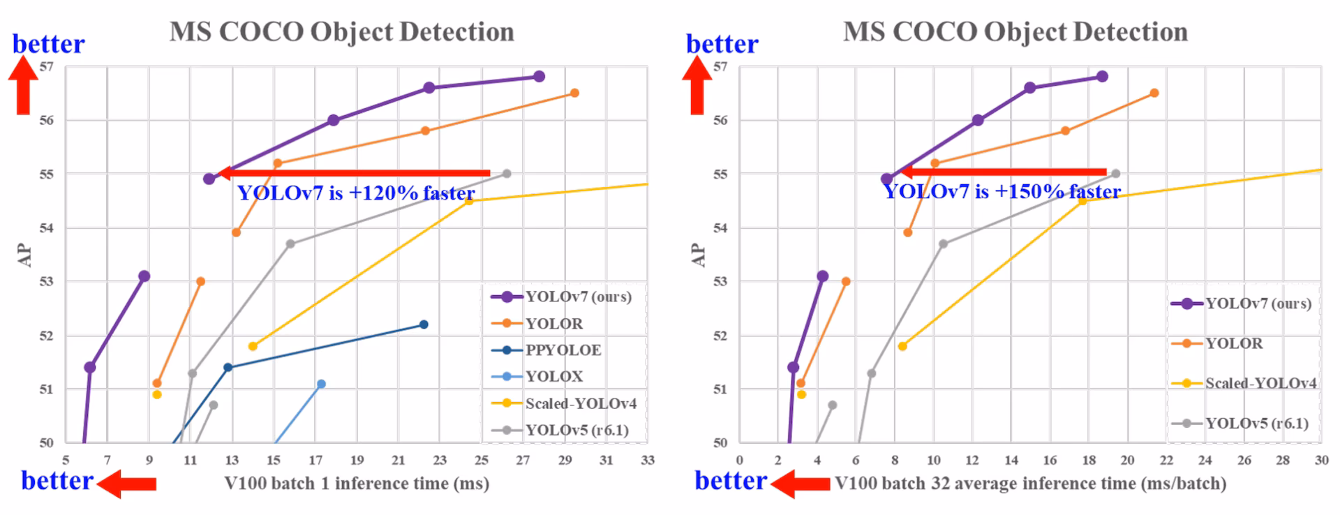
YOLOv7 于 2022 年 7 月发布,是当时实时目标检测领域的一次重大进展。它在 GPU V100 上达到了 56.8% 的 AP,在推出时树立了新的基准。YOLOv7 在速度和精度方面均优于当时的 YOLOR、YOLOX、Scaled-YOLOv4 和 YOLOv5 等目标检测模型。该模型是在 MS COCO 数据集上从零开始训练的,没有使用任何其他数据集或预训练权重。YOLOv7 的源代码可在 GitHub 上获取。请注意,像 YOLO11 和 YOLO26 这样的新模型已经在保持更高效率的同时实现了更高的精度。
Link to this sectionSOTA 目标检测器对比#
从 YOLO 对比表的结果中,我们了解到该方法在速度与精度之间实现了最全面的平衡。如果我们对比 YOLOv7-tiny-SiLU 和 YOLOv5-N (r6.1),我们的方法在 AP 方面快了 127 fps,精度高出 10.7%。此外,YOLOv7 在 161 fps 的帧率下拥有 51.4% 的 AP,而 AP 相同的 PPYOLOE-L 的帧率仅为 78 fps。在参数量方面,YOLOv7 比 PPYOLOE-L 少 41%。
如果我们对比推理速度为 114 fps 的 YOLOv7-X 和推理速度为 99 fps 的 YOLOv5-L (r6.1),YOLOv7-X 的 AP 可以提高 3.9%。如果将 YOLOv7-X 与同等规模的 YOLOv5-X (r6.1) 进行对比,YOLOv7-X 的推理速度要快 31 fps。此外,在参数量和计算量方面,与 YOLOv5-X (r6.1) 相比,YOLOv7-X 的参数量减少了 22%,计算量减少了 8%,但 AP 提高了 2.2% (来源)。
| 模型 | 参数 (M) | FLOPs (G) | 尺寸 (像素) | FPS | AP测试 / 验证 50-95 | AP测试 50 | AP测试 75 | AP测试 S | AP测试 M | AP测试 L |
|---|---|---|---|---|---|---|---|---|---|---|
| YOLOX-S | 9.0 | 26.8 | 640 | 102 | 40.5% / 40.5% | - | - | - | - | - |
| YOLOX-M | 25.3 | 73.8 | 640 | 81 | 47.2% / 46.9% | - | - | - | - | - |
| YOLOX-L | 54.2 | 155.6 | 640 | 69 | 50.1% / 49.7% | - | - | - | - | - |
| YOLOX-X | 99.1 | 281.9 | 640 | 58 | 51.5% / 51.1% | - | - | - | - | - |
| PPYOLOE-S | 7.9 | 17.4 | 640 | 208 | 43.1% / 42.7% | 60.5% | 46.6% | 23.2% | 46.4% | 56.9% |
| PPYOLOE-M | 23.4 | 49.9 | 640 | 123 | 48.9% / 48.6% | 66.5% | 53.0% | 28.6% | 52.9% | 63.8% |
| PPYOLOE-L | 52.2 | 110.1 | 640 | 78 | 51.4% / 50.9% | 68.9% | 55.6% | 31.4% | 55.3% | 66.1% |
| PPYOLOE-X | 98.4 | 206.6 | 640 | 45 | 52.2% / 51.9% | 69.9% | 56.5% | 33.3% | 56.3% | 66.4% |
| YOLOv5-N (r6.1) | 1.9 | 4.5 | 640 | 159 | - / 28.0% | - | - | - | - | - |
| YOLOv5-S (r6.1) | 7.2 | 16.5 | 640 | 156 | - / 37.4% | - | - | - | - | - |
| YOLOv5-M (r6.1) | 21.2 | 49.0 | 640 | 122 | - / 45.4% | - | - | - | - | - |
| YOLOv5-L (r6.1) | 46.5 | 109.1 | 640 | 99 | - / 49.0% | - | - | - | - | - |
| YOLOv5-X (r6.1) | 86.7 | 205.7 | 640 | 83 | - / 50.7% | - | - | - | - | - |
| YOLOR-CSP | 52.9 | 120.4 | 640 | 106 | 51.1% / 50.8% | 69.6% | 55.7% | 31.7% | 55.3% | 64.7% |
| YOLOR-CSP-X | 96.9 | 226.8 | 640 | 87 | 53.0% / 52.7% | 71.4% | 57.9% | 33.7% | 57.1% | 66.8% |
| YOLOv7-tiny-SiLU | 6.2 | 13.8 | 640 | 286 | 38.7% / 38.7% | 56.7% | 41.7% | 18.8% | 42.4% | 51.9% |
| YOLOv7 | 36.9 | 104.7 | 640 | 161 | 51.4% / 51.2% | 69.7% | 55.9% | 31.8% | 55.5% | 65.0% |
| YOLOv7-X | 71.3 | 189.9 | 640 | 114 | 53.1% / 52.9% | 71.2% | 57.8% | 33.8% | 57.1% | 67.4% |
| YOLOv5-N6 (r6.1) | 3.2 | 18.4 | 1280 | 123 | - / 36.0% | - | - | - | - | - |
| YOLOv5-S6 (r6.1) | 12.6 | 67.2 | 1280 | 122 | - / 44.8% | - | - | - | - | - |
| YOLOv5-M6 (r6.1) | 35.7 | 200.0 | 1280 | 90 | - / 51.3% | - | - | - | - | - |
| YOLOv5-L6 (r6.1) | 76.8 | 445.6 | 1280 | 63 | - / 53.7% | - | - | - | - | - |
| YOLOv5-X6 (r6.1) | 140.7 | 839.2 | 1280 | 38 | - / 55.0% | - | - | - | - | - |
| YOLOR-P6 | 37.2 | 325.6 | 1280 | 76 | 53.9% / 53.5% | 71.4% | 58.9% | 36.1% | 57.7% | 65.6% |
| YOLOR-W6 | 79.8 | 453.2 | 1280 | 66 | 55.2% / 54.8% | 72.7% | 60.5% | 37.7% | 59.1% | 67.1% |
| YOLOR-E6 | 115.8 | 683.2 | 1280 | 45 | 55.8% / 55.7% | 73.4% | 61.1% | 38.4% | 59.7% | 67.7% |
| YOLOR-D6 | 151.7 | 935.6 | 1280 | 34 | 56.5% / 56.1% | 74.1% | 61.9% | 38.9% | 60.4% | 68.7% |
| YOLOv7-W6 | 70.4 | 360.0 | 1280 | 84 | 54.9% / 54.6% | 72.6% | 60.1% | 37.3% | 58.7% | 67.1% |
| YOLOv7-E6 | 97.2 | 515.2 | 1280 | 56 | 56.0% / 55.9% | 73.5% | 61.2% | 38.0% | 59.9% | 68.4% |
| YOLOv7-D6 | 154.7 | 806.8 | 1280 | 44 | 56.6% / 56.3% | 74.0% | 61.8% | 38.8% | 60.1% | 69.5% |
| YOLOv7-E6E | 151.7 | 843.2 | 1280 | 36 | 56.8% / 56.8% | 74.4% | 62.1% | 39.3% | 60.5% | 69.0% |
Link to this section概述#
实时目标检测是许多 computer vision 系统的重要组成部分,包括多 object tracking、自动驾驶、robotics 和 medical image analysis。近年来,实时目标检测的发展重点在于设计高效的架构并提高各种 CPU、GPU 和神经网络处理单元 (NPU) 的推理速度。YOLOv7 支持从边缘设备到云端的移动 GPU 和 GPU 设备。
与专注于架构优化的传统实时目标检测器不同,YOLOv7 引入了对训练过程优化的关注。这包括旨在提高目标检测精度而不增加推理成本的模块和优化方法,这一概念被称为“可训练的免费赠品 (trainable bag-of-freebies)”。
Link to this section主要特性#
YOLOv7 引入了几个关键特性:
-
模型重参数化:YOLOv7 提出了一种规划好的重参数化模型,这是一种利用梯度传播路径的概念,适用于不同网络层的策略。
-
动态标签分配:使用多个输出层对模型进行训练带来了一个新问题:“如何为不同分支的输出分配动态目标?”为了解决这个问题,YOLOv7 引入了一种称为粗到细引导标签分配 (coarse-to-fine lead guided label assignment) 的新标签分配方法。
-
扩展和复合缩放:YOLOv7 为实时目标检测器提出了“扩展”和“复合缩放”方法,可以有效利用参数和计算资源。
-
效率:YOLOv7 提出的方法可以有效地将最先进的实时目标检测器的参数减少约 40%,计算量减少约 50%,并具有更快的推理速度和更高的检测精度。
Link to this section使用示例#
Ultralytics 不发布 yolov7.pt 预训练权重或 ultralytics/cfg/models/v7/ YAML 文件,并且 Ultralytics Python 软件包不支持 YOLOv7 的原生 PyTorch 训练和推理。不过,你可以通过将其导出为 ONNX 或 TensorRT,将 upstream YOLOv7 repository 中训练的 YOLOv7 检查点引入 Ultralytics,如下所示。
Link to this sectionONNX 导出#
要在 Ultralytics 中使用 YOLOv7 ONNX 模型:
-
(可选)安装 Ultralytics 并导出 ONNX 模型以自动安装所需的依赖项:
pip install ultralytics yolo export model=yolo26n.pt format=onnx -
使用 YOLOv7 repo 中的导出器导出所需的 YOLOv7 模型:
git clone https://github.com/WongKinYiu/yolov7 cd yolov7 python export.py --weights yolov7-tiny.pt --grid --end2end --simplify --topk-all 100 --iou-thres 0.65 --conf-thres 0.35 --img-size 640 640 --max-wh 640 -
使用以下脚本修改 ONNX 模型图以使其与 Ultralytics 兼容:
import numpy as np import onnx from onnx import helper, numpy_helper # Load the ONNX model model_path = "yolov7/yolov7-tiny.onnx" # Replace with your model path model = onnx.load(model_path) graph = model.graph # Fix input shape to batch size 1 input_shape = graph.input[0].type.tensor_type.shape input_shape.dim[0].dim_value = 1 # Define the output of the original model original_output_name = graph.output[0].name # Create slicing nodes sliced_output_name = f"{original_output_name}_sliced" # Define initializers for slicing (remove the first value) start = numpy_helper.from_array(np.array([1], dtype=np.int64), name="slice_start") end = numpy_helper.from_array(np.array([7], dtype=np.int64), name="slice_end") axes = numpy_helper.from_array(np.array([1], dtype=np.int64), name="slice_axes") steps = numpy_helper.from_array(np.array([1], dtype=np.int64), name="slice_steps") graph.initializer.extend([start, end, axes, steps]) slice_node = helper.make_node( "Slice", inputs=[original_output_name, "slice_start", "slice_end", "slice_axes", "slice_steps"], outputs=[sliced_output_name], name="SliceNode", ) graph.node.append(slice_node) # Define segment slicing seg1_start = numpy_helper.from_array(np.array([0], dtype=np.int64), name="seg1_start") seg1_end = numpy_helper.from_array(np.array([4], dtype=np.int64), name="seg1_end") seg2_start = numpy_helper.from_array(np.array([4], dtype=np.int64), name="seg2_start") seg2_end = numpy_helper.from_array(np.array([5], dtype=np.int64), name="seg2_end") seg3_start = numpy_helper.from_array(np.array([5], dtype=np.int64), name="seg3_start") seg3_end = numpy_helper.from_array(np.array([6], dtype=np.int64), name="seg3_end") graph.initializer.extend([seg1_start, seg1_end, seg2_start, seg2_end, seg3_start, seg3_end]) # Create intermediate tensors for segments segment_1_name = f"{sliced_output_name}_segment1" segment_2_name = f"{sliced_output_name}_segment2" segment_3_name = f"{sliced_output_name}_segment3" # Add segment slicing nodes graph.node.extend( [ helper.make_node( "Slice", inputs=[sliced_output_name, "seg1_start", "seg1_end", "slice_axes", "slice_steps"], outputs=[segment_1_name], name="SliceSegment1", ), helper.make_node( "Slice", inputs=[sliced_output_name, "seg2_start", "seg2_end", "slice_axes", "slice_steps"], outputs=[segment_2_name], name="SliceSegment2", ), helper.make_node( "Slice", inputs=[sliced_output_name, "seg3_start", "seg3_end", "slice_axes", "slice_steps"], outputs=[segment_3_name], name="SliceSegment3", ), ] ) # Concatenate the segments concat_output_name = f"{sliced_output_name}_concat" concat_node = helper.make_node( "Concat", inputs=[segment_1_name, segment_3_name, segment_2_name], outputs=[concat_output_name], axis=1, name="ConcatSwapped", ) graph.node.append(concat_node) # Reshape to [1, -1, 6] reshape_shape = numpy_helper.from_array(np.array([1, -1, 6], dtype=np.int64), name="reshape_shape") graph.initializer.append(reshape_shape) final_output_name = f"{concat_output_name}_batched" reshape_node = helper.make_node( "Reshape", inputs=[concat_output_name, "reshape_shape"], outputs=[final_output_name], name="AddBatchDimension", ) graph.node.append(reshape_node) # Get the shape of the reshaped tensor shape_node_name = f"{final_output_name}_shape" shape_node = helper.make_node( "Shape", inputs=[final_output_name], outputs=[shape_node_name], name="GetShapeDim", ) graph.node.append(shape_node) # Extract the second dimension dim_1_index = numpy_helper.from_array(np.array([1], dtype=np.int64), name="dim_1_index") graph.initializer.append(dim_1_index) second_dim_name = f"{final_output_name}_dim1" gather_node = helper.make_node( "Gather", inputs=[shape_node_name, "dim_1_index"], outputs=[second_dim_name], name="GatherSecondDim", ) graph.node.append(gather_node) # Subtract from 100 to determine how many values to pad target_size = numpy_helper.from_array(np.array([100], dtype=np.int64), name="target_size") graph.initializer.append(target_size) pad_size_name = f"{second_dim_name}_padsize" sub_node = helper.make_node( "Sub", inputs=["target_size", second_dim_name], outputs=[pad_size_name], name="CalculatePadSize", ) graph.node.append(sub_node) # Build the [2, 3] pad array: # 1st row -> [0, 0, 0] (no padding at the start of any dim) # 2nd row -> [0, pad_size, 0] (pad only at the end of the second dim) pad_starts = numpy_helper.from_array(np.array([0, 0, 0], dtype=np.int64), name="pad_starts") graph.initializer.append(pad_starts) zero_scalar = numpy_helper.from_array(np.array([0], dtype=np.int64), name="zero_scalar") graph.initializer.append(zero_scalar) pad_ends_name = "pad_ends" concat_pad_ends_node = helper.make_node( "Concat", inputs=["zero_scalar", pad_size_name, "zero_scalar"], outputs=[pad_ends_name], axis=0, name="ConcatPadEnds", ) graph.node.append(concat_pad_ends_node) pad_values_name = "pad_values" concat_pad_node = helper.make_node( "Concat", inputs=["pad_starts", pad_ends_name], outputs=[pad_values_name], axis=0, name="ConcatPadStartsEnds", ) graph.node.append(concat_pad_node) # Create Pad operator to pad with zeros pad_output_name = f"{final_output_name}_padded" pad_constant_value = numpy_helper.from_array( np.array([0.0], dtype=np.float32), name="pad_constant_value", ) graph.initializer.append(pad_constant_value) pad_node = helper.make_node( "Pad", inputs=[final_output_name, pad_values_name, "pad_constant_value"], outputs=[pad_output_name], mode="constant", name="PadToFixedSize", ) graph.node.append(pad_node) # Update the graph's final output to [1, 100, 6] new_output_type = onnx.helper.make_tensor_type_proto( elem_type=graph.output[0].type.tensor_type.elem_type, shape=[1, 100, 6] ) new_output = onnx.helper.make_value_info(name=pad_output_name, type_proto=new_output_type) # Replace the old output with the new one graph.output.pop() graph.output.extend([new_output]) # Save the modified model onnx.save(model, "yolov7-ultralytics.onnx") -
然后,你可以加载修改后的 ONNX 模型并在 Ultralytics 中正常运行推理:
from ultralytics import ASSETS, YOLO

model = YOLO("yolov7-ultralytics.onnx", task="detect")

results = model(ASSETS / "bus.jpg")
Link to this sectionTensorRT 导出#
-
按照 ONNX Export 部分中的步骤 1-2 进行操作。
-
安装
TensorRTPython 软件包:pip install tensorrt -
运行以下脚本将修改后的 ONNX 模型转换为 TensorRT 引擎:
from ultralytics.utils.export import export_engine export_engine("yolov7-ultralytics.onnx", half=True) -
在 Ultralytics 中加载并运行该模型:
from ultralytics import ASSETS, YOLO

model = YOLO("yolov7-ultralytics.engine", task="detect")

results = model(ASSETS / "bus.jpg")
Link to this section引用与致谢#
我们感谢 YOLOv7 作者在实时目标检测领域做出的重大贡献:
@inproceedings{wang2023yolov7,
  title={YOLOv7: Trainable Bag-of-Freebies Sets New State-of-the-Art for Real-Time Object Detectors},
  author={Wang, Chien-Yao and Bochkovskiy, Alexey and Liao, Hong-Yuan Mark},
  booktitle={Proceedings of the IEEE/CVF conference on Computer Vision and Pattern Recognition (CVPR)},
  pages={7464--7475},
  year={2023}
}
YOLOv7 官方论文发表在 CVF 2023 Open Access 上,预印本可在 arXiv 上查阅。作者已将其工作公开,代码库可在 GitHub 上访问。我们感谢他们在推动该领域发展并使更广泛的社区能够获得其成果方面所做的努力。
Link to this section常见问题解答#
Link to this section什么是 YOLOv7,为什么它被认为是实时 object detection 的突破?#
YOLOv7 发布于 2022 年 7 月,是一款重要的实时目标检测模型,在发布时实现了出色的速度和精度。它在参数使用和推理速度方面都超越了当时的 YOLOX、YOLOv5 和 PPYOLOE 等模型。YOLOv7 的显著特点包括其模型重参数化和动态标签分配,这些特点在不增加推理成本的情况下优化了性能。有关其架构和与其他最先进目标检测器比较指标的更多技术细节,请参阅 YOLOv7 paper。
Link to this sectionYOLOv7 如何改进了 YOLOv4 和 YOLOv5 等以前的 YOLO 模型?#
YOLOv7 引入了几项创新,包括模型重参数化和动态标签分配,这些创新增强了训练过程并提高了推理精度。与 YOLOv5 相比,YOLOv7 显著提高了速度和精度。例如,与 YOLOv5-X 相比,YOLOv7-X 的精度提高了 2.2%,参数减少了 22%。详细比较可以在性能表 YOLOv7 comparison with SOTA object detectors 中找到。
Link to this section我可以使用 Ultralytics 工具和平台使用 YOLOv7 吗?#
目前,Ultralytics 仅支持 YOLOv7 ONNX 和 TensorRT 推理。要使用 Ultralytics 运行 YOLOv7 的 ONNX 和 TensorRT 导出版本,请查看 Usage Examples 部分。
Link to this section如何使用我的数据集训练自定义 YOLOv7 模型?#
要安装和训练自定义 YOLOv7 模型,请按照以下步骤操作:
-
克隆 YOLOv7 存储库:
git clone https://github.com/WongKinYiu/yolov7 -
导航到克隆的目录并安装依赖项:
cd yolov7 pip install -r requirements.txt -
根据存储库中提供的 usage instructions 准备你的数据集并配置模型参数。 如需进一步指导,请访问 YOLOv7 GitHub 存储库以获取最新信息和更新。
-
训练后,你可以将模型导出为 ONNX 或 TensorRT,以便在 Ultralytics 中使用,如 Usage Examples 所示。
Link to this sectionYOLOv7 引入的关键特性和优化是什么?#
YOLOv7 提供了几项彻底改变实时目标检测的关键特性:
- 模型重参数化:通过优化梯度传播路径增强了模型的性能。
- 动态标签分配:使用粗到细引导方法为不同分支的输出分配动态目标,从而提高精度。
- 扩展和复合缩放:高效利用参数和计算资源,为各种实时应用扩展模型。
- 效率:与其他最先进的模型相比,参数数量减少了 40%,计算量减少了 50%,同时实现了更快的推理速度。
有关这些特性的更多详细信息,请参阅 YOLOv7 Overview 部分。