YOLOv7: 훈련 가능한 Bag-of-Freebies

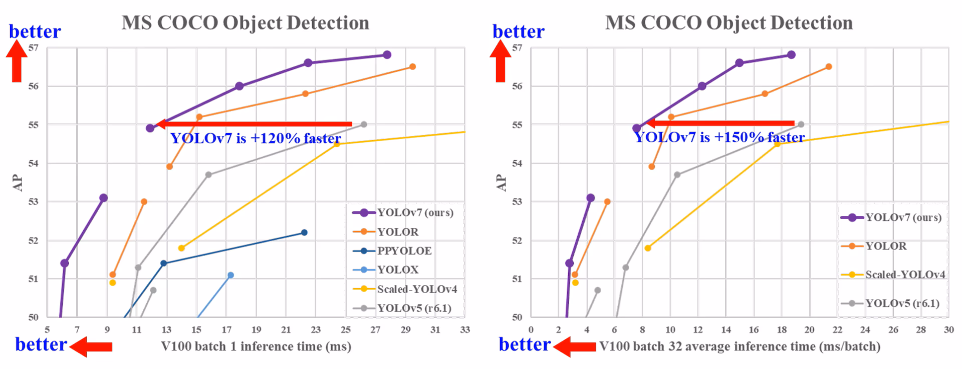
2022년 7월에 출시된 YOLOv7은 출시 당시 실시간 객체 detect 분야에서 중요한 진전을 이루었습니다. GPU V100에서 56.8% AP를 달성하여 도입 당시 새로운 벤치마크를 세웠습니다. YOLOv7은 YOLOR, YOLOX, Scaled-YOLOv4, YOLOv5와 같은 동시대 객체 detect 모델들을 속도와 정확도 면에서 능가했습니다. 이 모델은 다른 데이터셋이나 사전 훈련된 가중치를 사용하지 않고 MS COCO 데이터셋으로 처음부터 훈련되었습니다. YOLOv7의 소스 코드는 GitHub에서 확인할 수 있습니다. 참고로, YOLO11 및 YOLO26과 같은 최신 모델들은 이후 향상된 효율성으로 더 높은 정확도를 달성했습니다.

SOTA 객체 감지기 비교

YOLO 비교표의 결과에서 제안된 방법이 종합적으로 최고의 속도-정확도 트레이드오프를 가짐을 알 수 있습니다. YOLOv7-tiny-SiLU를 YOLOv5-N (r6.1)과 비교하면, 저희 방법은 127 fps 더 빠르고 AP에서 10.7% 더 정확합니다. 또한, YOLOv7은 161 fps의 프레임 속도에서 51.4% AP를 달성하는 반면, 동일한 AP를 가진 PPYOLOE-L은 78 fps의 프레임 속도만을 가집니다. 파라미터 사용 측면에서 YOLOv7은 PPYOLOE-L보다 41% 적습니다.

114 fps 추론 속도를 가진 YOLOv7-X를 99 fps 추론 속도를 가진 YOLOv5-L (r6.1)과 비교하면, YOLOv7-X는 AP를 3.9% 향상시킬 수 있습니다. YOLOv7-X를 유사한 규모의 YOLOv5-X (r6.1)와 비교하면, YOLOv7-X의 추론 속도는 31 fps 더 빠릅니다. 또한, 파라미터 및 연산량 측면에서 YOLOv7-X는 YOLOv5-X (r6.1)에 비해 파라미터를 22%, 연산량을 8% 줄이면서도 AP를 2.2% 향상시킵니다 (출처).

개요

실시간 객체 detect는 다중 객체 track, 자율 주행, 로봇 공학, 의료 영상 분석을 포함한 많은 컴퓨터 비전 시스템의 중요한 구성 요소입니다. 최근 몇 년 동안 실시간 객체 detect 개발은 효율적인 아키텍처 설계와 다양한 CPU, GPU 및 신경 처리 장치(NPU)의 추론 속도 향상에 중점을 두었습니다. YOLOv7은 엣지에서 클라우드에 이르기까지 모바일 GPU 및 GPU 장치를 모두 지원합니다.

아키텍처 최적화에 중점을 둔 기존의 실시간 객체 detect기와 달리, YOLOv7은 훈련 프로세스 최적화에 중점을 둡니다. 이는 추론 비용을 증가시키지 않으면서 객체 detect의 정확도를 향상시키도록 설계된 모듈 및 최적화 방법을 포함하며, 이는 "trainable bag-of-freebies"라는 개념으로 알려져 있습니다.

주요 기능

YOLOv7은 몇 가지 주요 기능을 소개합니다:

1. 모델 재매개변수화: YOLOv7은 기울기 전파 경로의 개념을 통해 다양한 네트워크의 레이어에 적용 가능한 전략인 계획된 재매개변수화 모델을 제안합니다.

2. 동적 레이블 할당: 다중 출력 레이어를 가진 모델의 훈련은 "서로 다른 브랜치의 출력에 동적 타겟을 어떻게 할당할 것인가?"라는 새로운 문제를 제기합니다. 이 문제를 해결하기 위해 YOLOv7은 coarse-to-fine lead guided label assignment라는 새로운 레이블 할당 방식을 도입합니다.

3. 확장 및 복합 스케일링: YOLOv7은 매개변수와 연산을 효과적으로 활용할 수 있는 실시간 객체 detect기에 대해 "확장(extend)" 및 "복합 스케일링(compound scaling)" 방식을 제안합니다.

4. 효율성: YOLOv7이 제안하는 방식은 최첨단 실시간 객체 detect기의 매개변수를 약 40%, 연산량을 50% 가량 효과적으로 줄일 수 있으며, 더 빠른 추론 속도와 더 높은 detect 정확도를 제공합니다.

사용 예시

이 글을 쓰는 시점에는 Ultralytics는 YOLOv7에 대해 ONNX 및 TensorRT 추론만 지원합니다.

ONNX 내보내기

Ultralytics와 함께 YOLOv7 ONNX 모델을 사용하려면:

1. (선택 사항) 필요한 종속성이 자동으로 설치되도록 Ultralytics를 설치하고 ONNX 모델을 내보냅니다.

   pip install ultralytics
   yolo export model=yolo26n.pt format=onnx
   

2. YOLOv7 repo의 익스포터를 사용하여 원하는 YOLOv7 모델을 내보내십시오:

   git clone https://github.com/WongKinYiu/yolov7
   cd yolov7
   python export.py --weights yolov7-tiny.pt --grid --end2end --simplify --topk-all 100 --iou-thres 0.65 --conf-thres 0.35 --img-size 640 640 --max-wh 640
   

3. 다음 스크립트를 사용하여 Ultralytics와 호환되도록 ONNX 모델 그래프를 수정합니다.

   import numpy as np
   import onnx
   from onnx import helper, numpy_helper
   
   # Load the ONNX model
   model_path = "yolov7/yolov7-tiny.onnx"  # Replace with your model path
   model = onnx.load(model_path)
   graph = model.graph
   
   # Fix input shape to batch size 1
   input_shape = graph.input[0].type.tensor_type.shape
   input_shape.dim[0].dim_value = 1
   
   # Define the output of the original model
   original_output_name = graph.output[0].name
   
   # Create slicing nodes
   sliced_output_name = f"{original_output_name}_sliced"
   
   # Define initializers for slicing (remove the first value)
   start = numpy_helper.from_array(np.array([1], dtype=np.int64), name="slice_start")
   end = numpy_helper.from_array(np.array([7], dtype=np.int64), name="slice_end")
   axes = numpy_helper.from_array(np.array([1], dtype=np.int64), name="slice_axes")
   steps = numpy_helper.from_array(np.array([1], dtype=np.int64), name="slice_steps")
   
   graph.initializer.extend([start, end, axes, steps])
   
   slice_node = helper.make_node(
       "Slice",
       inputs=[original_output_name, "slice_start", "slice_end", "slice_axes", "slice_steps"],
       outputs=[sliced_output_name],
       name="SliceNode",
   )
   graph.node.append(slice_node)
   
   # Define segment slicing
   seg1_start = numpy_helper.from_array(np.array([0], dtype=np.int64), name="seg1_start")
   seg1_end = numpy_helper.from_array(np.array([4], dtype=np.int64), name="seg1_end")
   seg2_start = numpy_helper.from_array(np.array([4], dtype=np.int64), name="seg2_start")
   seg2_end = numpy_helper.from_array(np.array([5], dtype=np.int64), name="seg2_end")
   seg3_start = numpy_helper.from_array(np.array([5], dtype=np.int64), name="seg3_start")
   seg3_end = numpy_helper.from_array(np.array([6], dtype=np.int64), name="seg3_end")
   
   graph.initializer.extend([seg1_start, seg1_end, seg2_start, seg2_end, seg3_start, seg3_end])
   
   # Create intermediate tensors for segments
   segment_1_name = f"{sliced_output_name}_segment1"
   segment_2_name = f"{sliced_output_name}_segment2"
   segment_3_name = f"{sliced_output_name}_segment3"
   
   # Add segment slicing nodes
   graph.node.extend(
       [
           helper.make_node(
               "Slice",
               inputs=[sliced_output_name, "seg1_start", "seg1_end", "slice_axes", "slice_steps"],
               outputs=[segment_1_name],
               name="SliceSegment1",
           ),
           helper.make_node(
               "Slice",
               inputs=[sliced_output_name, "seg2_start", "seg2_end", "slice_axes", "slice_steps"],
               outputs=[segment_2_name],
               name="SliceSegment2",
           ),
           helper.make_node(
               "Slice",
               inputs=[sliced_output_name, "seg3_start", "seg3_end", "slice_axes", "slice_steps"],
               outputs=[segment_3_name],
               name="SliceSegment3",
           ),
       ]
   )
   
   # Concatenate the segments
   concat_output_name = f"{sliced_output_name}_concat"
   concat_node = helper.make_node(
       "Concat",
       inputs=[segment_1_name, segment_3_name, segment_2_name],
       outputs=[concat_output_name],
       axis=1,
       name="ConcatSwapped",
   )
   graph.node.append(concat_node)
   
   # Reshape to [1, -1, 6]
   reshape_shape = numpy_helper.from_array(np.array([1, -1, 6], dtype=np.int64), name="reshape_shape")
   graph.initializer.append(reshape_shape)
   
   final_output_name = f"{concat_output_name}_batched"
   reshape_node = helper.make_node(
       "Reshape",
       inputs=[concat_output_name, "reshape_shape"],
       outputs=[final_output_name],
       name="AddBatchDimension",
   )
   graph.node.append(reshape_node)
   
   # Get the shape of the reshaped tensor
   shape_node_name = f"{final_output_name}_shape"
   shape_node = helper.make_node(
       "Shape",
       inputs=[final_output_name],
       outputs=[shape_node_name],
       name="GetShapeDim",
   )
   graph.node.append(shape_node)
   
   # Extract the second dimension
   dim_1_index = numpy_helper.from_array(np.array([1], dtype=np.int64), name="dim_1_index")
   graph.initializer.append(dim_1_index)
   
   second_dim_name = f"{final_output_name}_dim1"
   gather_node = helper.make_node(
       "Gather",
       inputs=[shape_node_name, "dim_1_index"],
       outputs=[second_dim_name],
       name="GatherSecondDim",
   )
   graph.node.append(gather_node)
   
   # Subtract from 100 to determine how many values to pad
   target_size = numpy_helper.from_array(np.array([100], dtype=np.int64), name="target_size")
   graph.initializer.append(target_size)
   
   pad_size_name = f"{second_dim_name}_padsize"
   sub_node = helper.make_node(
       "Sub",
       inputs=["target_size", second_dim_name],
       outputs=[pad_size_name],
       name="CalculatePadSize",
   )
   graph.node.append(sub_node)
   
   # Build the [2, 3] pad array:
   # 1st row -> [0, 0, 0] (no padding at the start of any dim)
   # 2nd row -> [0, pad_size, 0] (pad only at the end of the second dim)
   pad_starts = numpy_helper.from_array(np.array([0, 0, 0], dtype=np.int64), name="pad_starts")
   graph.initializer.append(pad_starts)
   
   zero_scalar = numpy_helper.from_array(np.array([0], dtype=np.int64), name="zero_scalar")
   graph.initializer.append(zero_scalar)
   
   pad_ends_name = "pad_ends"
   concat_pad_ends_node = helper.make_node(
       "Concat",
       inputs=["zero_scalar", pad_size_name, "zero_scalar"],
       outputs=[pad_ends_name],
       axis=0,
       name="ConcatPadEnds",
   )
   graph.node.append(concat_pad_ends_node)
   
   pad_values_name = "pad_values"
   concat_pad_node = helper.make_node(
       "Concat",
       inputs=["pad_starts", pad_ends_name],
       outputs=[pad_values_name],
       axis=0,
       name="ConcatPadStartsEnds",
   )
   graph.node.append(concat_pad_node)
   
   # Create Pad operator to pad with zeros
   pad_output_name = f"{final_output_name}_padded"
   pad_constant_value = numpy_helper.from_array(
       np.array([0.0], dtype=np.float32),
       name="pad_constant_value",
   )
   graph.initializer.append(pad_constant_value)
   
   pad_node = helper.make_node(
       "Pad",
       inputs=[final_output_name, pad_values_name, "pad_constant_value"],
       outputs=[pad_output_name],
       mode="constant",
       name="PadToFixedSize",
   )
   graph.node.append(pad_node)
   
   # Update the graph's final output to [1, 100, 6]
   new_output_type = onnx.helper.make_tensor_type_proto(
       elem_type=graph.output[0].type.tensor_type.elem_type, shape=[1, 100, 6]
   )
   new_output = onnx.helper.make_value_info(name=pad_output_name, type_proto=new_output_type)
   
   # Replace the old output with the new one
   graph.output.pop()
   graph.output.extend([new_output])
   
   # Save the modified model
   onnx.save(model, "yolov7-ultralytics.onnx")
   

4. 그런 다음 수정된 ONNX 모델을 로드하고 Ultralytics에서 정상적으로 추론을 실행할 수 있습니다.

   from ultralytics import ASSETS, YOLO
   
   model = YOLO("yolov7-ultralytics.onnx", task="detect")
   
   results = model(ASSETS / "bus.jpg")
   

TensorRT 내보내기

1. ONNX 내보내기 섹션의 1~2단계를 따르세요.

2. 다음을 설치합니다. TensorRT Python 패키지:

   pip install tensorrt
   

3. 수정된 ONNX 모델을 TensorRT 엔진으로 변환하려면 다음 스크립트를 실행합니다.

   from ultralytics.utils.export import export_engine
   
   export_engine("yolov7-ultralytics.onnx", half=True)
   

4. Ultralytics에서 모델을 로드하고 실행합니다.

   from ultralytics import ASSETS, YOLO
   
   model = YOLO("yolov7-ultralytics.engine", task="detect")
   
   results = model(ASSETS / "bus.jpg")
   

인용 및 감사의 말씀

실시간 객체 detect 분야에 크게 기여한 YOLOv7 저자들에게 감사를 표합니다:

@article{wang2022yolov7,
  title={YOLOv7: Trainable bag-of-freebies sets new state-of-the-art for real-time object detectors},
  author={Wang, Chien-Yao and Bochkovskiy, Alexey and Liao, Hong-Yuan Mark},
  journal={arXiv preprint arXiv:2207.02696},
  year={2022}
}

원본 YOLOv7 논문은 arXiv에서 찾아볼 수 있습니다. 저자들은 자신들의 작업을 공개적으로 이용할 수 있도록 했으며, 코드베이스는 GitHub에서 접근할 수 있습니다. 저자들의 분야 발전 노력과 더 넓은 커뮤니티에 대한 작업 공개에 감사드립니다.

FAQ

YOLOv7은 무엇이며, 실시간 객체 detect 분야에서 왜 획기적인 발전으로 평가받습니까?

2022년 7월에 출시된 YOLOv7은 출시 당시 뛰어난 속도와 정확도를 달성한 중요한 실시간 객체 detect 모델이었습니다. YOLOX, YOLOv5, PPYOLOE와 같은 동시대 모델들을 매개변수 사용량과 추론 속도 모두에서 능가했습니다. YOLOv7의 특징은 모델 재매개변수화와 동적 레이블 할당으로, 추론 비용을 늘리지 않고 성능을 최적화합니다. 아키텍처 및 다른 최첨단 객체 detect 모델과의 비교 지표에 대한 자세한 기술 정보는 YOLOv7 논문을 참조하십시오.

YOLOv7은 YOLOv4 및 YOLOv5와 같은 이전 YOLO 모델에 비해 어떻게 개선되었습니까?

YOLOv7은 모델 재매개변수화 및 동적 레이블 할당을 포함한 여러 혁신을 도입하여 훈련 프로세스를 향상시키고 추론 정확도를 개선합니다. YOLOv5와 비교하여 YOLOv7은 속도와 정확도를 크게 향상시킵니다. 예를 들어, YOLOv7-X는 YOLOv5-X에 비해 정확도를 2.2% 향상시키고 매개변수를 22% 줄입니다. 자세한 비교는 성능 표 YOLOv7과 SOTA 객체 detect기 비교에서 확인할 수 있습니다.

Ultralytics 도구 및 플랫폼에서 YOLOv7을 사용할 수 있습니까?

현재 Ultralytics는 YOLOv7 ONNX 및 TensorRT 추론만 지원합니다. Ultralytics와 함께 ONNX 및 TensorRT로 내보낸 YOLOv7 버전을 실행하려면 사용 예시 섹션을 확인하십시오.

내 데이터셋을 사용하여 사용자 지정 YOLOv7 모델을 어떻게 훈련합니까?

사용자 지정 YOLOv7 모델을 설치하고 훈련하려면 다음 단계를 따르십시오:

1. YOLOv7 저장소를 클론하십시오:

   git clone https://github.com/WongKinYiu/yolov7
   

2. 복제된 디렉토리로 이동하여 종속성을 설치합니다:

   cd yolov7
   pip install -r requirements.txt
   

3. 저장소에 제공된 사용 지침에 따라 데이터셋을 준비하고 모델 매개변수를 구성하십시오. 더 자세한 지침은 최신 정보 및 업데이트를 위해 YOLOv7 GitHub 저장소를 방문하십시오.

4. 학습 후 사용 예제에 표시된 대로 Ultralytics에서 사용하기 위해 모델을 ONNX 또는 TensorRT로 내보낼 수 있습니다.

YOLOv7에 도입된 주요 기능 및 최적화는 무엇입니까?

YOLOv7은 실시간 객체 detect에 혁명을 일으키는 몇 가지 주요 기능을 제공합니다:

• 모델 재파라미터화: 기울기 전파 경로를 최적화하여 모델의 성능을 향상시킵니다.
• 동적 레이블 할당: coarse-to-fine lead guided 방법을 사용하여 서로 다른 분기의 출력에 대한 동적 대상을 할당하여 정확도를 향상시킵니다.
• 확장 및 복합 스케일링: 다양한 실시간 애플리케이션을 위해 모델을 확장하기 위해 파라미터와 계산을 효율적으로 활용합니다.
• 효율성: 더 빠른 추론 속도를 달성하면서 다른 최첨단 모델에 비해 매개변수 수를 40% 줄이고 계산량을 50% 줄입니다.

이러한 기능에 대한 자세한 내용은 YOLOv7 개요 섹션을 참조하십시오.

5; 2 년 전에 생성됨 ✏️ 2 전에 업데이트됨

댓글