VOC探索の例


Ultralytics Explorer APIノートブックへようこそ。このノートブックでは、セマンティック検索、ベクトル検索、およびSQLクエリを使用してデータセットを探索するために利用できるリソースを紹介します。
試す yolo explorer (Explorer APIを搭載)
インストール ultralytics そして、実行します。 yolo explorer ターミナルで、ブラウザでカスタムクエリとセマンティック検索を実行します。
コミュニティノート ⚠️
〜の時点で ultralytics>=8.3.10、Ultralytics Explorerのサポートは非推奨になりました。同様の(そして拡張された)データセット探索機能は、以下で利用できます。 Ultralytics Platform.
セットアップ
インストール ultralytics および必要な 依存関係、次にソフトウェアとハードウェアを確認します。
!uv pip install ultralytics[explorer] openai
yolo checks
類似度検索
ベクトルの類似性検索の力を活用して、データセット内の類似したデータ点と、埋め込み空間でのそれらの距離を見つけます。与えられたデータセットとモデルのペアに対して、embeddingsテーブルを作成するだけです。これは一度だけ必要で、自動的に再利用されます。
exp = Explorer("VOC.yaml", model="yolo26n.pt")
exp.create_embeddings_table()
埋め込みテーブルが構築されたら、以下のいずれかの方法でセマンティック検索を実行できます。
- データセット内の特定のインデックス/インデックスリストに対して、例:
exp.get_similar(idx=[1, 10], limit=10) - データセットにない任意の画像/画像のリストに対して - exp.get_similar(img=["path/to/img1", "path/to/img2"], limit=10)。複数の入力がある場合、それらの埋め込みの集合が使用されます。
入力に最も類似したデータポイントを制限数だけ含むPandas DataFrameが、埋め込み空間におけるそれらの距離とともに取得されます。このデータセットを使用して、さらにフィルタリングを実行できます。
# Search dataset by index
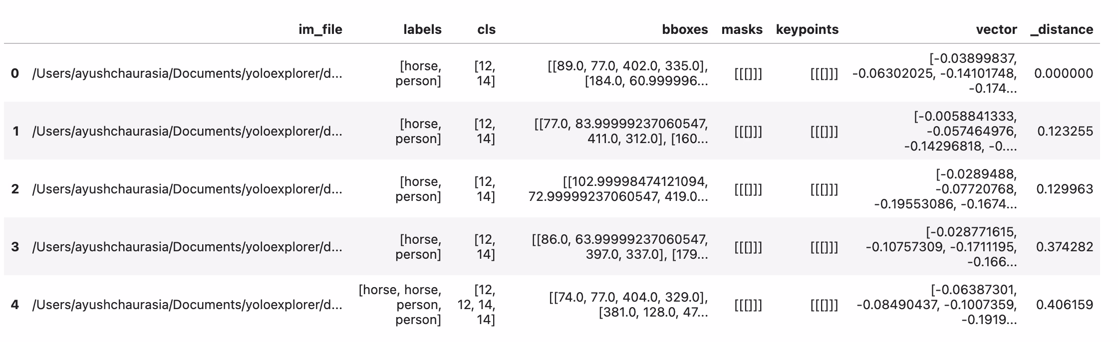
similar = exp.get_similar(idx=1, limit=10)
similar.head()
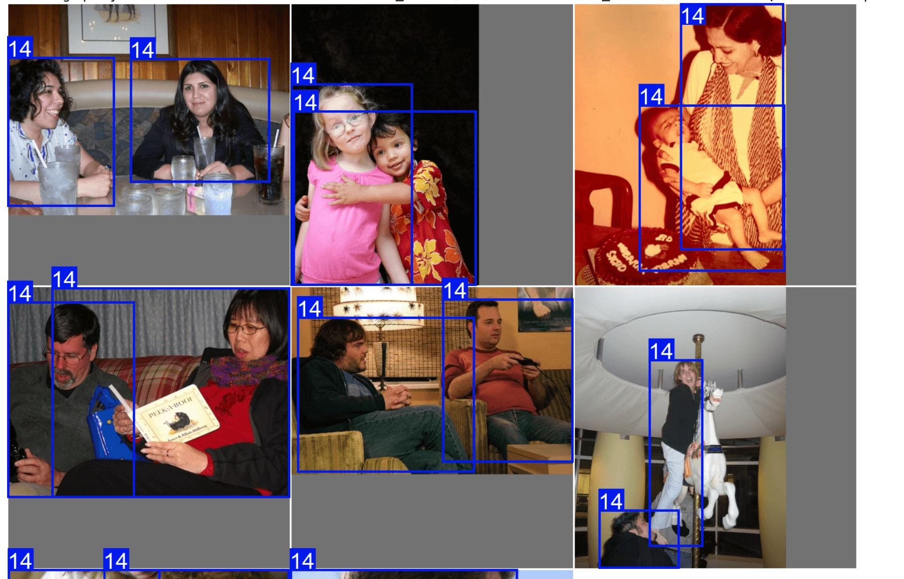
また、類似したサンプルを直接プロットすることもできます。 plot_similar util
exp.plot_similar(idx=6500, limit=20)
exp.plot_similar(idx=[100, 101], limit=10)  # Can also pass list of idxs or imgs

exp.plot_similar(img="https://ultralytics.com/images/bus.jpg", limit=10, labels=False)  # Can also pass external images
AIに質問:自然言語で検索またはフィルタリング
Explorerオブジェクトに表示したいデータポイントの種類をプロンプトとして与えることができ、その結果を含むDataFrameを返そうとします。LLMによって駆動されているため、常に正確であるとは限りません。その場合、以下を返します None.
df = exp.ask_ai("show me images containing more than 10 objects with at least 2 persons")
df.head(5)
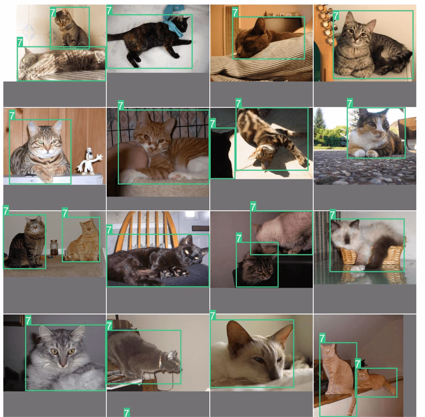
これらの結果をプロットするには、 plot_query_result ユーティリティを使用できます。例:
plt = plot_query_result(exp.ask_ai("show me 10 images containing exactly 2 persons"))
Image.fromarray(plt)
# plot
from PIL import Image
from ultralytics.data.explorer import plot_query_result

plt = plot_query_result(exp.ask_ai("show me 10 images containing exactly 2 persons"))
Image.fromarray(plt)
データセットに対してSQLクエリを実行
データセット内の特定の項目を調査したい場合があります。このため、ExplorerはSQLクエリの実行を可能にします。以下のいずれかの形式を受け入れます。
- 「WHERE」で始まるクエリは、すべての列を自動的に選択します。これはショートハンドクエリと考えることができます。
- どの列を選択するかを指定できる完全なクエリを記述することもできます。
これは、モデルのパフォーマンスと特定のデータポイントを調査するために使用できます。例:
- モデルが人間と犬が写っている画像を苦手とする場合を考えてみましょう。少なくとも2人の人間と少なくとも1匹の犬がいるポイントを選択するために、このようなクエリを作成できます。
SQLクエリとセマンティック検索を組み合わせて、特定の結果タイプに絞り込むことができます。
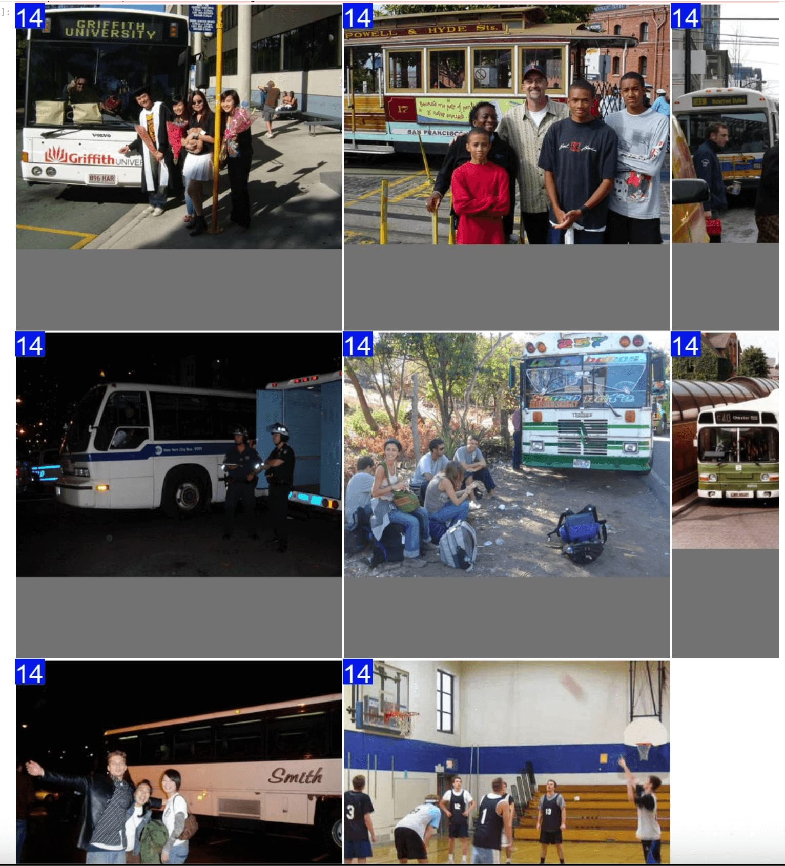
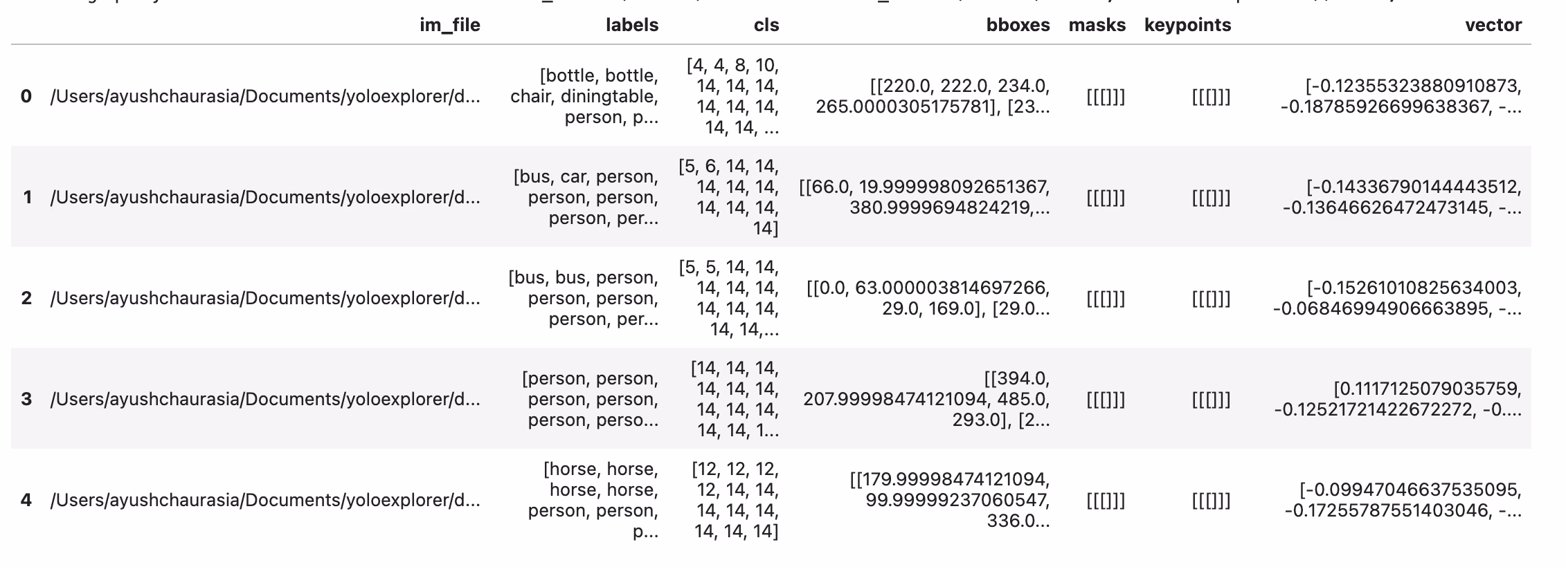
table = exp.sql_query("WHERE labels LIKE '%person, person%' AND labels LIKE '%dog%' LIMIT 10")
exp.plot_sql_query("WHERE labels LIKE '%person, person%' AND labels LIKE '%dog%' LIMIT 10", labels=True)
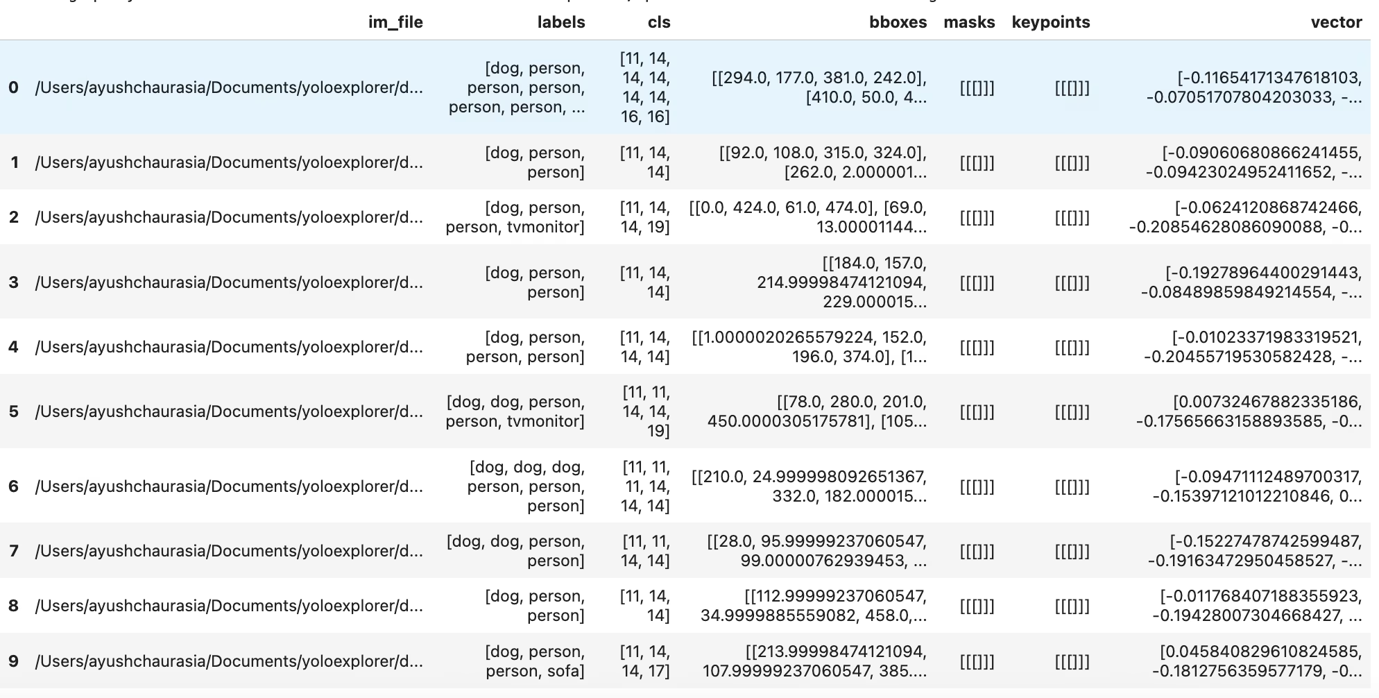
table = exp.sql_query("WHERE labels LIKE '%person, person%' AND labels LIKE '%dog%' LIMIT 10")
print(table)
類似性検索と同様に、sqlクエリを直接プロットするためのユーティリティも取得できます。 exp.plot_sql_query
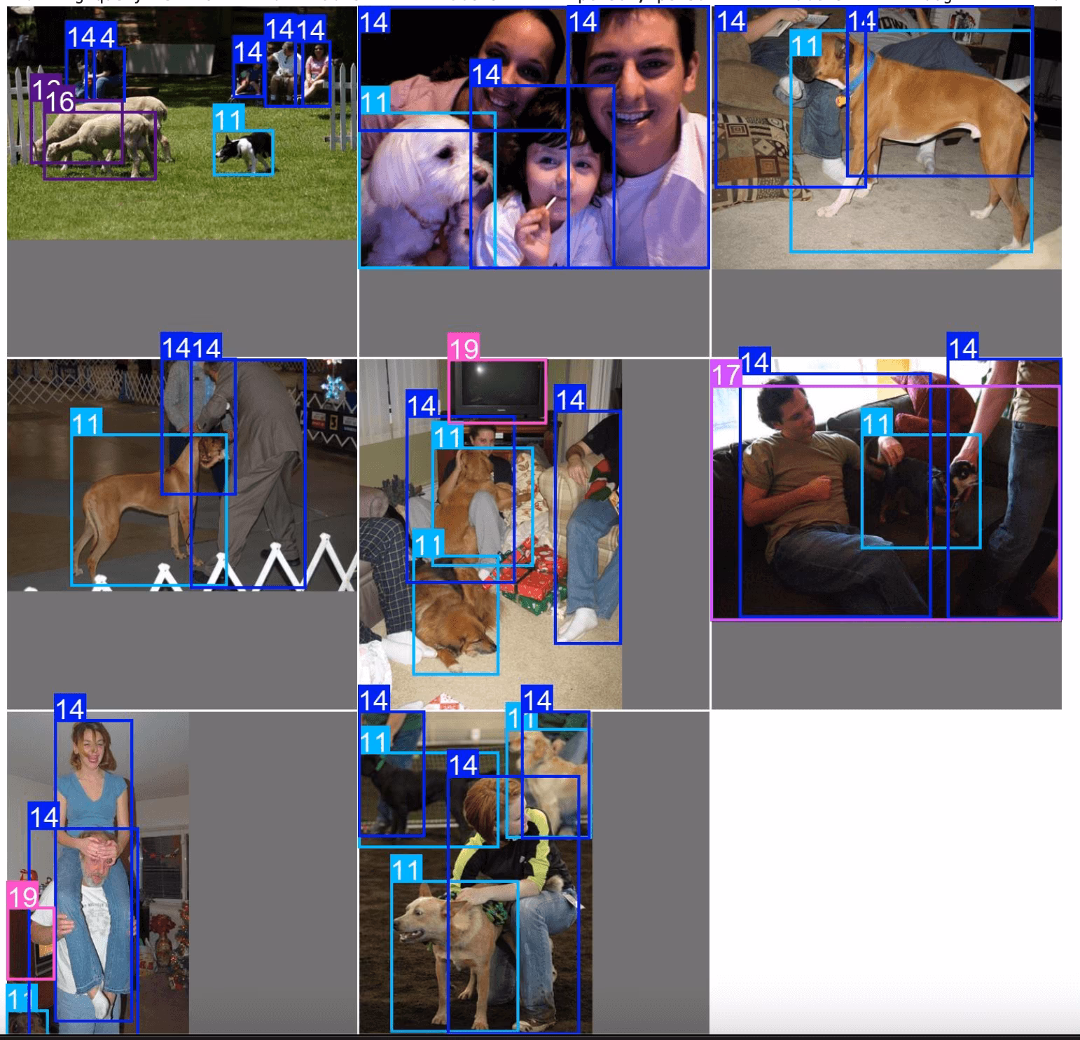
exp.plot_sql_query("WHERE labels LIKE '%person, person%' AND labels LIKE '%dog%' LIMIT 10", labels=True)
埋め込みテーブルの操作(高度)
Explorerは以下で動作します。 LanceDB テーブルを内部的に使用します。このテーブルには、以下を使用して直接アクセスできます。 Explorer.table オブジェクトと生のクエリを実行したり、事前および事後フィルターをプッシュダウンしたりできます。
table = exp.table
print(table.schema)
raw クエリの実行
Vector Searchは、データベースから最も近いベクトルを検索します。レコメンデーションシステムや検索エンジンでは、検索した製品と類似した製品を見つけることができます。LLMやその他のAIアプリケーションでは、各データポイントをいくつかのモデルから生成された埋め込みで表現でき、最も関連性の高い特徴を返します。
高次元ベクトル空間での探索は、クエリベクトルのK近傍(KNN)を見つけることです。
LanceDBにおけるMetricとは、ベクトルのペア間の距離を記述する方法です。現在、以下のメトリックがサポートされています。
- L2
- コサイン
- Dot Explorerの類似性検索は、デフォルトでL2を使用します。テーブルに対して直接クエリを実行したり、lance形式を使用してデータセットを管理するためのカスタムユーティリティを構築したりできます。利用可能なLanceDBテーブル操作の詳細については、ドキュメントを参照してください。
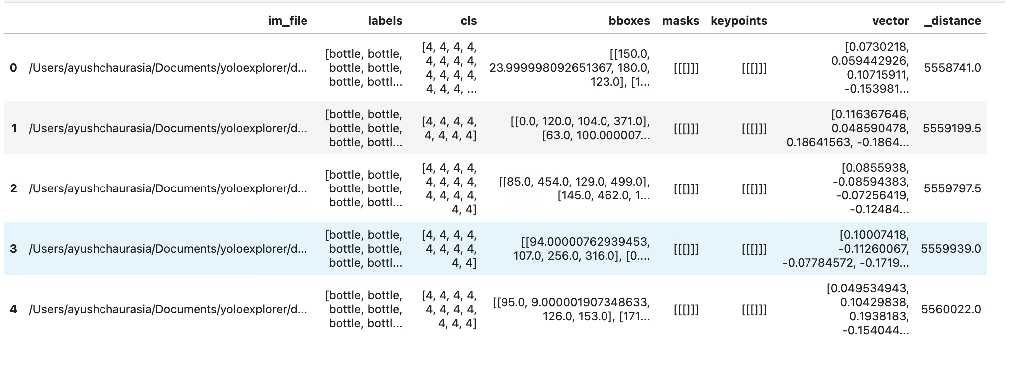
dummy_img_embedding = [i for i in range(256)]
table.search(dummy_img_embedding).limit(5).to_pandas()
一般的なデータ形式への相互変換
df = table.to_pandas()
pa_table = table.to_arrow()
埋め込みの操作
lancedbテーブルから生の埋め込みにアクセスし、分析することができます。画像の埋め込みは列に保存されています vector
import numpy as np

embeddings = table.to_pandas()["vector"].tolist()
embeddings = np.array(embeddings)
散布図
埋め込みを分析する際の予備的なステップの1つは、次元削減を介して2D空間にプロットすることです。例を試してみましょう
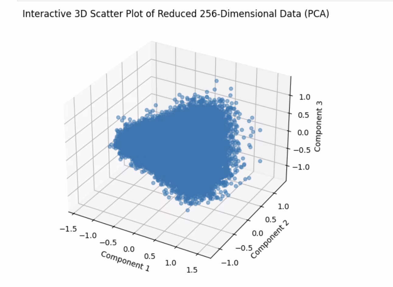
import matplotlib.pyplot as plt
from sklearn.decomposition import PCA  # pip install scikit-learn

# Reduce dimensions using PCA to 3 components for visualization in 3D
pca = PCA(n_components=3)
reduced_data = pca.fit_transform(embeddings)

# Create a 3D scatter plot using Matplotlib's Axes3D
fig = plt.figure(figsize=(8, 6))
ax = fig.add_subplot(111, projection="3d")

# Scatter plot
ax.scatter(reduced_data[:, 0], reduced_data[:, 1], reduced_data[:, 2], alpha=0.5)
ax.set_title("3D Scatter Plot of Reduced 256-Dimensional Data (PCA)")
ax.set_xlabel("Component 1")
ax.set_ylabel("Component 2")
ax.set_zlabel("Component 3")

plt.show()
類似度指標
埋め込みテーブルを利用した操作の簡単な例を以下に示します。Explorerには以下が付属しています。 similarity_index operation-
- 各データポイントがデータセットの残りの部分とどれだけ類似しているかを推定しようとします。
- これは、生成された埋め込み空間において、現在の画像に対してmax_distよりも近い画像埋め込みがいくつあるかを、一度にtop_k個の類似画像を考慮して数えることによって行われます。
特定のデータセット、モデルについて max_dist & top_k 一度生成された類似度インデックスは再利用されます。データセットが変更された場合、または単に類似度インデックスを再生成する必要がある場合は、以下を渡すことができます。 force=True。ベクトル検索やSQL検索と同様に、これも直接プロットするためのユーティリティが付属しています。
sim_idx = exp.similarity_index(max_dist=0.2, top_k=0.01)
exp.plot_similarity_index(max_dist=0.2, top_k=0.01)
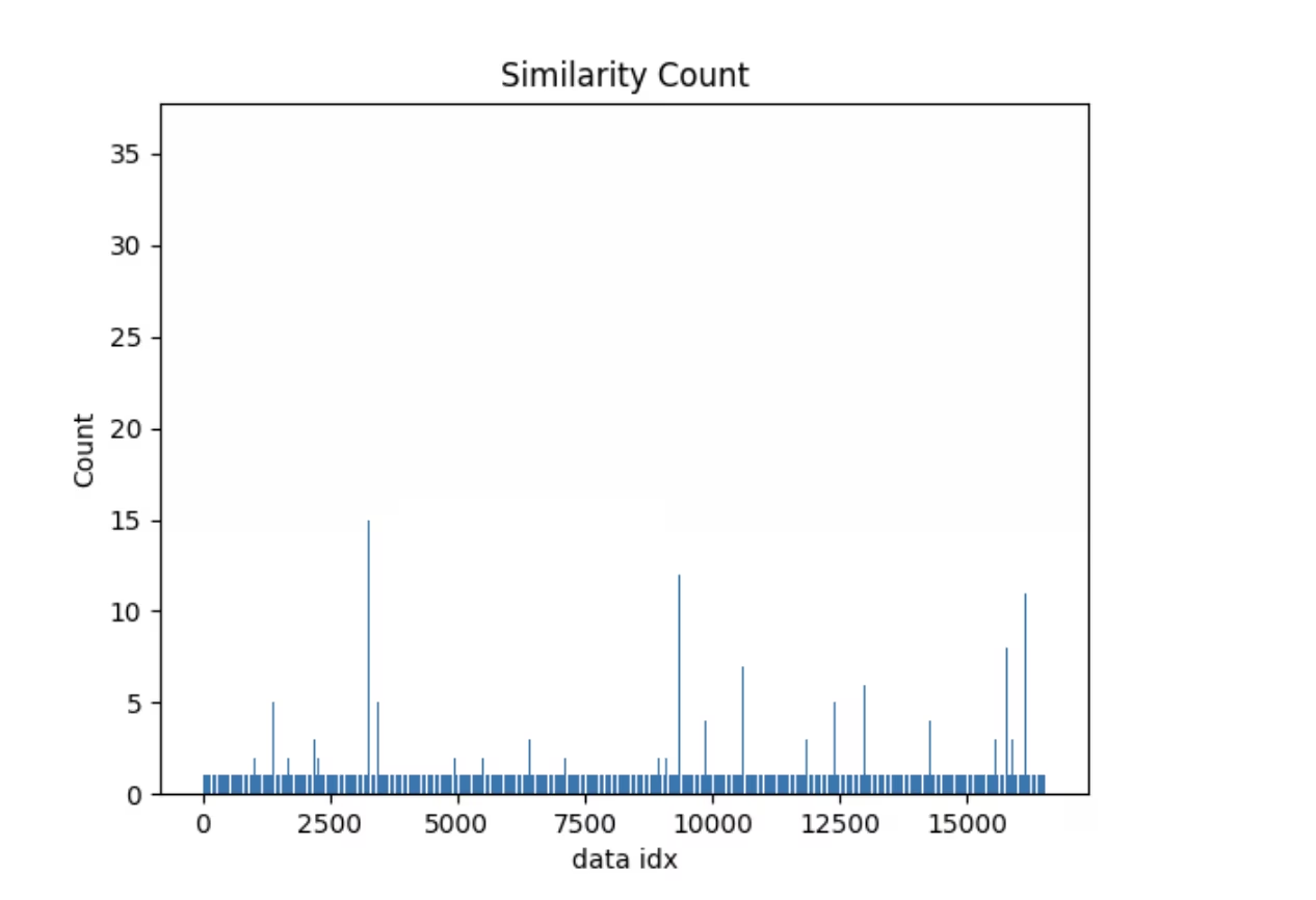
まずはプロットを見てみましょう
exp.plot_similarity_index(max_dist=0.2, top_k=0.01)
次に、操作の出力を見てみましょう。
sim_idx = exp.similarity_index(max_dist=0.2, top_k=0.01, force=False)

sim_idx
類似性カウントが30を超えるデータポイントを確認し、それらに類似した画像をプロットするクエリを作成してみましょう。
import numpy as np

sim_count = np.array(sim_idx["count"])
sim_idx["im_file"][sim_count > 30]
次のようなものが表示されるはずです。
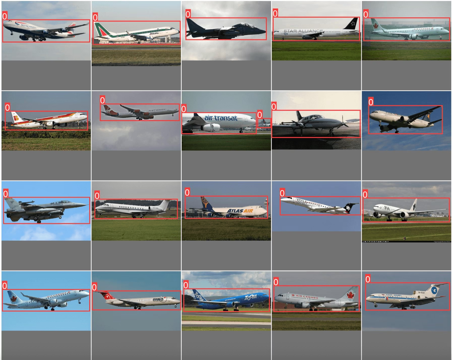
exp.plot_similar(idx=[7146, 14035]) # Using avg embeddings of 2 images


