Ultralytics YOLO26 ile Analitik
Ultralytics YOLO26 ile analitik, nesne algılama ve izleme sonuçlarını gerçek zamanlı grafiklere dönüştürür; böylece nesne sayılarının video kareleri boyunca nasıl değiştiğini takip edebilirsin. Bu kılavuz dört veri görselleştirme türünü kapsar — çizgi grafikleri, çubuk grafikler, pasta grafikleri ve alan grafikleri — ve ortak Python ve CLI örnekleriyle bunlar arasında nasıl geçiş yapılacağını gösterir.
İzle: Ultralytics ile Analitik Grafikler Nasıl Oluşturulur | Çizgi Grafikleri, Çubuk Grafikler, Alan Grafikleri ve Pasta Grafikleri
Görsel Örnekler#
| Çizgi Grafiği | Çubuk Grafik | Pasta Grafiği |
|---|---|---|
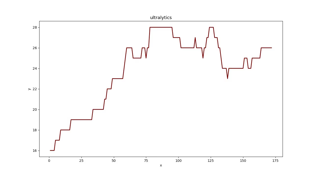 | 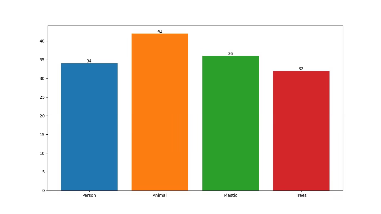 | 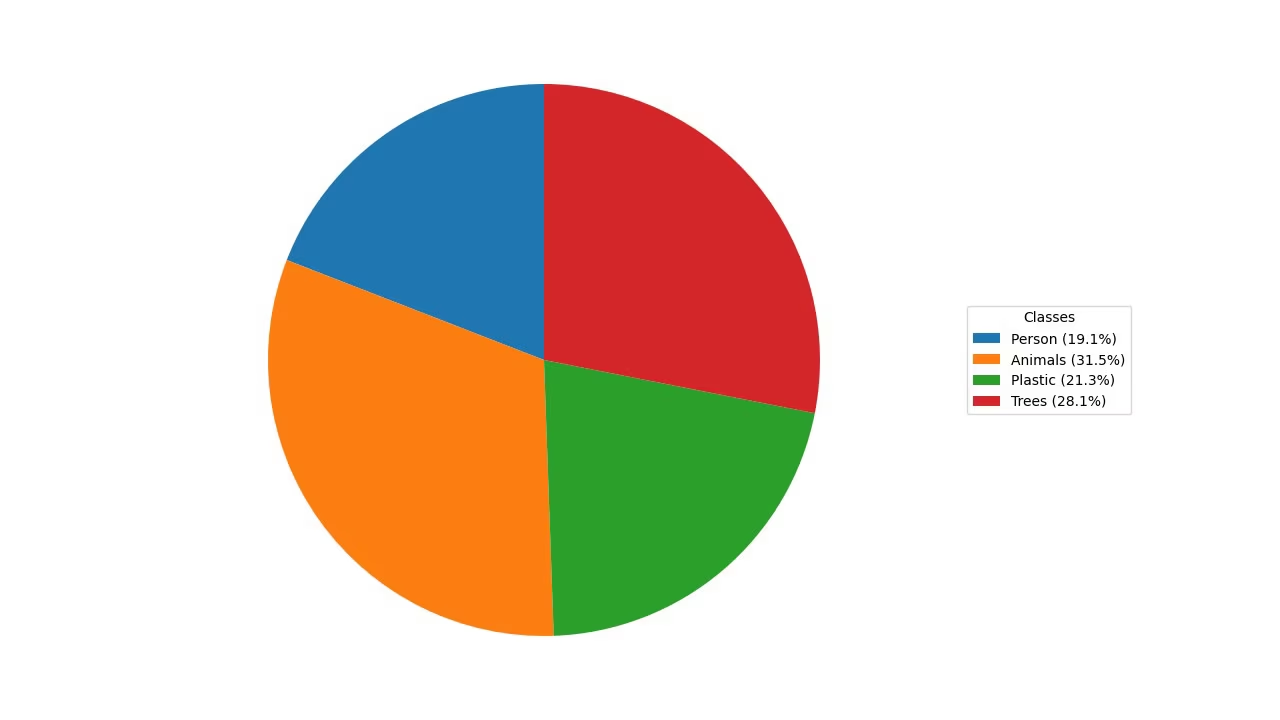 |
Algılama Verileri Neden Görselleştirilir?#
- Çizgi grafikleri, kısa ve uzun dönemlerdeki değişiklikleri izlemek ve aynı dönemde birden fazla gruptaki değişiklikleri karşılaştırmak için idealdir.
- Çubuk grafikler, farklı kategorilerdeki miktarları karşılaştırmak ve bir kategoriyle sayısal değeri arasındaki ilişkileri göstermek için uygundur.
- Pasta grafikleri, kategoriler arasındaki oranları göstermek ve bir bütünün parçalarını görselleştirmek için etkilidir.
- Alan grafikleri, çizgi grafiğinin altını doldurarak sınıf başına nesne sayılarının zamana göre bir bakışta daha kolay okunmasını sağlar.
Analitik Grafikleri Oluştur#
Videonu Analytics çözümüne aktar ve analytics_type ile bir grafik seç. Çözüm her karede algılama ve izleme işlemlerini çalıştırır, ardından doğrudan çıktı videosuna yazabileceğin (varsayılan olarak) 1280×720 boyutunda bir grafik oluşturur. Tek bir bağımsız değişkenle "line", "bar", "pie" ve "area" arasında geçiş yap.
yolo solutions analytics show=True

# Pass the source
yolo solutions analytics source="path/to/video.mp4"

# Generate the pie chart
yolo solutions analytics analytics_type="pie" show=True

# Generate the bar plots
yolo solutions analytics analytics_type="bar" show=True

# Generate the area plots
yolo solutions analytics analytics_type="area" show=True
Analytics Bağımsız Değişkenleri#
Analitik bağımsız değişkenlerini gösteren bir tablo:
| Bağımsız değişken | Tür | Varsayılan | Açıklama |
|---|---|---|---|
model | str | None | Ultralytics YOLO model dosyasının yolu. |
analytics_type | str | 'line' | Grafik türü; yani line, bar, area veya pie. |
figsize | tuple[float, float] | (12.8, 7.2) | Analytics grafikleri için inç cinsinden şekil boyutu; (12.8, 7.2), 1280×720 boyutunda bir kare oluşturur. |
line_width | int | 2 | Çözümün çizdiği kutular, anahtar noktalar ve sayılar için çizgi kalınlığı. |
verbose | bool | True | Çözümün her kare için girdi şekli, sınıf sayıları ve işleme hızına ilişkin günlüğünü etkinleştirir. İzleme çağrısının kendisi her zaman sessizdir. |
Analytics çözümünde track bağımsız değişkenlerini de kullanabilirsin.
| Bağımsız değişken | Tür | Varsayılan | Açıklama |
|---|---|---|---|
tracker | str | 'tracktrack.yaml' | Kullanılacak izleme algoritmasını belirtir. Yerleşik seçenekler: botsort.yaml, bytetrack.yaml, ocsort.yaml, deepocsort.yaml, fasttrack.yaml, tracktrack.yaml. |
conf | float | 0.25 | Algılamalar için güven eşiğini belirler; düşük değerler daha fazla nesnenin izlenmesine olanak tanır ancak yanlış pozitifleri de içerebilir. |
iou | float | 0.5 | Çakışan algılamaları filtrelemek için Kesişim-Birleşim Oranı (IoU) eşiğini belirler. |
classes | list | None | Sonuçları sınıf dizinine göre filtreler. Örneğin, classes=[0, 2, 3] yalnızca belirtilen sınıfları izler. |
device | str | None | Çıkarım için kullanılacak cihazı belirtir (ör. cpu, cuda:0 veya 0). Kullanıcıların model yürütme için CPU, belirli bir GPU veya başka hesaplama cihazları arasında seçim yapmasına olanak tanır. |
imgsz | int or tuple | 640 | Hedef çıkarım görüntü boyutu: kare görüntüler için bir tam sayı veya bir (height, width) çifti. Boyutlar model adım değerine göre ayarlanır. |
max_det | int | 300 | Yoğun sahnelerde bir çözümün işleyeceği nesne sayısını sınırlamak için izleme öncesinde kare başına tutulan en yüksek algılama sayısı. |
quantize | int or str | None | Çıkarım hassasiyeti: CPU dışında PyTorch ve TorchScript modelleri için 16 (FP16) veya 32/unset (FP32); diğer biçimler, model yapıtının ve çalışma zamanının seçtiği hassasiyeti kullanır. Kullanımdan kaldırılan half argümanının yerini alır. |
Ayrıca aşağıdaki görselleştirme bağımsız değişkenleri de desteklenir:
| Bağımsız değişken | Tür | Varsayılan | Açıklama |
|---|---|---|---|
show | bool | False | True ise açıklama eklenmiş görüntüleri veya videoları bir pencerede gösterir. Geliştirme veya test sırasında anında görsel geri bildirim almak için kullanışlıdır. |
Sonuç#
Farklı görselleştirme türlerini ne zaman ve nasıl kullanacağını anlamak, etkili veri analizi için çok önemlidir. Çizgi grafikleri, çubuk grafikleri, pasta grafikleri ve alan grafikleri, verinin anlattıklarını daha açık ve etkili biçimde aktarmana yardımcı olabilecek temel araçlardır. Ultralytics YOLO26 Analytics çözümü, nesne algılama ve izleme sonuçlarından bu görselleştirmeleri oluşturmanın basitleştirilmiş bir yolunu sunarak görsel verilerinden anlamlı içgörüler çıkarmanı kolaylaştırır.
Sık Sorulan Sorular#
Ultralytics YOLO26 Analitik ile çizgi grafiği oluşturmak için şu adımları izle:
- Bir YOLO26 modeli yükle ve video dosyanı aç.
Analyticssınıfınıanalytics_type="line"ile başlat.- Nesne sayıları gibi verilerle çizgi grafiğini güncellemek için her karede çözümü çağırarak video kareleri üzerinde yineleme yap.
- Grafiği kaydetmek için
results.plot_imöğesini bir çıktı videosuna yaz.
Başlangıç noktası olarak yukarıdaki Python örneğini kullan — örnek tüm kare döngüsünü zaten çalıştırıyor ve varsayılan
analytics_typebir çizgi grafiği.Çubuk grafik oluşturmak için Ultralytics YOLO26 kullanmanın çeşitli avantajları vardır:
- Gerçek Zamanlı Veri Görselleştirme: Dinamik güncellemeler için nesne algılama sonuçlarını çubuk grafiklere entegre et.
- Kullanım Kolaylığı: Basit API ve işlevler, uygulamayı ve verileri görselleştirmeyi kolaylaştırır.
- Özelleştirme: Başlıkları, etiketleri, renkleri ve daha fazlasını özel gereksinimlerine göre düzenle.
- Verimlilik: Büyük miktarda veriyi verimli biçimde işle ve video işleme sırasında grafikleri gerçek zamanlı güncelle.
Çubuk grafik oluşturmak için yukarıdaki Python örneğinde
analytics_type="bar"ayarını yap — kare döngüsünün geri kalanı aynıdır. Önizleme için Görsel Örnekler bölümüne bak.Ultralytics YOLO26, şu nedenlerle pasta grafikleri oluşturmak için mükemmel bir seçenektir:
- Nesne Algılama ile Entegrasyon: Anında içgörü elde etmek için nesne algılama sonuçlarını doğrudan pasta grafiklerine entegre et.
- Kullanıcı Dostu API: Az miktarda kodla kolayca kurulur ve kullanılır.
- Özelleştirilebilirlik: Renkler, etiketler ve daha fazlası için çeşitli özelleştirme seçenekleri sunar.
- Gerçek Zamanlı Güncellemeler: Verileri gerçek zamanlı işle ve görselleştir; bu, video analitiği projeleri için idealdir.
Pasta grafiği oluşturmak için yukarıdaki Python örneğinde
analytics_type="pie"ayarını yap. Daha fazla bilgi için kılavuzdaki Görsel Örnekler bölümüne başvur.Evet. İzleme,
Analyticsçözümüne yerleşik olarak gelir: birden fazla nesneyi gerçek zamanlı olarak izler ve her 30 karede bir izlenen nesnelerin verileriyle grafiği yeniler; böylece çizgi grafikleri, çubuk grafikler, pasta grafikleri ve alan grafikleri canlı sayıları yansıtır. Yukarıdaki Python örneğindeki kare döngüsü tam olarak bunu yapar. Temel izleme işlevselliği hakkında bilgi edinmek için İzleme bölümüne bak.Ultralytics YOLO26, çeşitli nedenlerle OpenCV ve TensorFlow gibi diğer nesne algılama çözümlerinden ayrılır:
- Son Teknoloji Doğruluk: YOLO26; nesne algılama, örnek segmentasyonu, anlamsal segmentasyon ve sınıflandırma görevlerinde üstün doğruluk sunar.
- Kullanım Kolaylığı: Kullanıcı dostu API, kapsamlı kodlama gerektirmeden hızlı uygulama ve entegrasyon olanağı sağlar.
- Gerçek Zamanlı Performans: Yüksek hızlı çıkarım için optimize edilmiştir ve gerçek zamanlı uygulamalara uygundur.
- Çeşitli Uygulamalar: Çoklu nesne izlemeyi, özel model eğitimini ve ONNX, TensorRT ve CoreML gibi farklı biçimlere dışa aktarmayı destekler.
- Kapsamlı Belgeler: Kullanıcılara her adımda yol gösterecek kapsamlı belgeler ve blog kaynakları sunar.


Yorumlar17
Bir soru sor, sonuçlarını paylaş veya başka birine yardım et.
 User
Hello @glenn-jocher How we can optimize/modify the code for YOLO predict, so it can also give final compiled result of prediction as graph. In case of counting objects/cells classed as different categories in images stored in a root folder. Not just the images with the prediction boxes.
yolo train model=yolo11n.pt data=coco8.yaml epochs=100 imgsz=640
yolo predict model=yolo11n.pt source=path/to/bus.jpg
Like the count graph YOLO makes after training or bar/pie chart?
Thanks
- User
@pderrenger Greetings
- User
Hello,
In relation to the above question, will this code work?
#!/usr/bin/env python3 """ yolo_predict_results.py
Run YOLO predictions on a single image or a directory of images, save annotated images, export per-image and aggregate counts to CSV, and save plots (aggregate bar chart and optional stacked per-image bar chart).
Requirements: pip install ultralytics pandas matplotlib pillow
Usage (recommended - command line): # Single image python yolo_predict_results.py --model /path/to/yolo11n.pt --source /path/to/bus.jpg --output results --save-annotated --plot-aggregate
# Directory (batch)
python yolo_predict_results.py --model /path/to/yolo11n.pt --source /path/to/images_dir --output results --save-annotated --plot-per-image --plot-aggregate
This file includes clearly highlighted comments showing exactly where to set your model path and images directory if you prefer to hardcode them in the script instead of using CLI args. """
import argparse from collections import Counter from pathlib import Path import sys
import numpy as np import pandas as pd import matplotlib.pyplot as plt from PIL import Image
try: from ultralytics import YOLO except Exception as e: print("Please install ultralytics (pip install ultralytics).") raise
IMAGE_EXTS = {".jpg", ".jpeg", ".png", ".bmp", ".tif", ".tiff", ".webp"}
def find_images(directory: Path): return [str(p) for p in sorted(directory.rglob("*")) if p.suffix.lower() in IMAGE_EXTS]
def predict_images(model, paths, conf=0.25, imgsz=640, device=None, save_annotated=False, out_dir=None): """ Run prediction per-image (keeps mapping simple). Returns list of dicts: {'file': path, 'counts': Counter, 'total': int} """ out_dir = Path(out_dir) if out_dir is not None else None annotated_dir = (out_dir / "annotated") if (save_annotated and out_dir is not None) else None if annotated_dir: annotated_dir.mkdir(parents=True, exist_ok=True)
results = []
for p in paths:
    print(f"Predicting: {p}")
    res_list = model.predict(source=p, conf=conf, imgsz=imgsz, device=device, verbose=False)
    if not res_list:
        print(f"Warning: no result for {p}")
        continue
    r = res_list[0]

    counts = Counter()
    try:
        box_cls = getattr(r.boxes, "cls", None)
        if box_cls is not None:
            try:
                arr = box_cls.cpu().numpy()
            except Exception:
                arr = np.array(box_cls)
            arr = arr.astype(int).flatten()
            for c in arr:
                name = model.names.get(int(c), str(int(c)))
                counts[name] += 1
    except Exception as e:
        print(f"Warning: could not parse classes for {p}: {e}")

    total = sum(counts.values())
    results.append({"file": p, "counts": counts, "total": total})

    if save_annotated and annotated_dir:
        try:
            ann = r.plot()
            if isinstance(ann, np.ndarray):
                img_out = Image.fromarray(ann)
            else:
                img_out = ann
            out_path = annotated_dir / (Path(p).stem + "_annotated" + Path(p).suffix)
            img_out.save(out_path)
        except Exception as e:
            print(f"Warning: failed to save annotated image for {p}: {e}")

return results
def build_dataframe(summary): all_classes = set() for row in summary: all_classes.update(row["counts"].keys()) classes = sorted(all_classes)
rows = []
for row in summary:
    data = {cls: row["counts"].get(cls, 0) for cls in classes}
    data["file"] = row["file"]
    data["total"] = row["total"]
    rows.append(data)

if not rows:
    # Return empty dataframe
    df = pd.DataFrame(columns=["file", "total"] + classes)
else:
    df = pd.DataFrame(rows)
    cols = ["file"] + classes + ["total"]
    df = df[cols]
return df, classes
def save_csvs(summary, out_dir: Path): df, classes = build_dataframe(summary) out_dir.mkdir(parents=True, exist_ok=True) csv1 = out_dir / "counts_per_image.csv" df.to_csv(csv1, index=False) print(f"Saved per-image counts to: {csv1}")
agg = Counter()
for r in summary:
    agg.update(r["counts"])
agg_series = pd.Series(dict(agg)).sort_values(ascending=False)
csv2 = out_dir / "aggregate_counts.csv"
agg_series.to_csv(csv2, header=["count"])
print(f"Saved aggregate counts to: {csv2}")
return df, classes, agg
def plot_aggregate(agg_counter, out_path: Path): names = list(agg_counter.keys()) counts = [agg_counter[n] for n in names] fig, ax = plt.subplots(figsize=(max(6, len(names) * 0.6), 5)) ax.bar(names, counts, color="tab:blue") ax.set_ylabel("Count") ax.set_title("Aggregate object counts") plt.xticks(rotation=45, ha="right") plt.tight_layout() out_path.parent.mkdir(parents=True, exist_ok=True) fig.savefig(out_path) plt.close(fig) print(f"Saved aggregate plot to: {out_path}")
def plot_stacked_per_image(df: pd.DataFrame, classes, out_path: Path, top_n=50): if df.empty: print("No per-image data to plot.") return plot_df = df.copy() if top_n and len(plot_df) > top_n: plot_df = plot_df.sort_values("total", ascending=False).head(top_n) x = plot_df["file"].apply(lambda p: Path(p).name).tolist() bottoms = np.zeros(len(plot_df)) fig, ax = plt.subplots(figsize=(max(8, len(x) * 0.6), 6)) for cls in classes: vals = plot_df[cls].values ax.bar(x, vals, bottom=bottoms, label=cls) bottoms += vals ax.set_ylabel("Counts") ax.set_title("Per-image stacked counts") ax.legend(bbox_to_anchor=(1.05, 1), loc="upper left") plt.xticks(rotation=45, ha="right") plt.tight_layout() out_path.parent.mkdir(parents=True, exist_ok=True) fig.savefig(out_path) plt.close(fig) print(f"Saved per-image stacked plot to: {out_path}")
def main(): ap = argparse.ArgumentParser(description="YOLO predict -> save CSV + plots") ap.add_argument("--model", required=False, help="Path to YOLO model (.pt) (e.g., yolo11n.pt)") ap.add_argument("--source", required=False, help="Image file or directory of images") ap.add_argument("--output", required=False, help="Output directory", default="results") ap.add_argument("--conf", type=float, default=0.25, help="Confidence threshold") ap.add_argument("--imgsz", type=int, default=640, help="Image size for inference") ap.add_argument("--device", type=str, default=None, help="Device (e.g., 0 or 'cpu')") ap.add_argument("--save-annotated", action="store_true", help="Save annotated images") ap.add_argument("--plot-per-image", action="store_true", help="Save stacked per-image plot") ap.add_argument("--plot-aggregate", action="store_true", help="Save aggregate bar chart") ap.add_argument("--top-n", type=int, default=50, help="Top N images for per-image plot when many images")
# Parse CLI args (recommended usage)
args = ap.parse_args()

# -------------------------------------------------------------------------
# HIGHLIGHT 1: If you want to hardcode paths, replace the `args = ap.parse_args()` line
# with the block below. Edit the two highlighted lines inside the block:
#    model="..."   <-- SET YOUR MODEL FILE PATH HERE
#    source="..."  <-- SET YOUR IMAGE FILE OR IMAGES DIRECTORY PATH HERE
#
# Example (UNCOMMENT and EDIT, then COMMENT OUT or REMOVE the args = ap.parse_args() above):
#
# args = argparse.Namespace(
#     model="/path/to/yolo11n.pt",       # <<< HIGHLIGHT: set model path here (absolute or relative)
#     source="/path/to/images_or_image", # <<< HIGHLIGHT: set image file or images directory path here
#     output="results",
#     conf=0.25,
#     imgsz=640,
#     device=None,
#     save_annotated=True,
#     plot_per_image=True,
#     plot_aggregate=True,
#     top_n=50
# )
# -------------------------------------------------------------------------

# -------------------------------------------------------------------------
# HIGHLIGHT 2: If you prefer using the command-line, supply these two args when
# running the script:
#   --model /path/to/yolo11n.pt
#   --source /path/to/images_or_image
# These correspond to the variables used below: args.model and args.source
# -------------------------------------------------------------------------

if not args.model or not args.source:
    print("Error: --model and --source are required (or hardcode them in the script).")
    print("Example:")
    print("  python yolo_predict_results.py --model /path/to/yolo11n.pt --source /path/to/images --output results --save-annotated --plot-aggregate")
    sys.exit(1)

model_path = Path(args.model)
source = Path(args.source)
out_dir = Path(args.output)
out_dir.mkdir(parents=True, exist_ok=True)

print(f"Loading model: {model_path}")
model = YOLO(str(model_path))

if source.is_dir():
    files = find_images(source)
    if not files:
        print(f"No images found under {source}")
        sys.exit(1)
elif source.is_file():
    files = [str(source)]
else:
    print(f"Source path not found: {source}")
    sys.exit(1)

summary = predict_images(
    model=model,
    paths=files,
    conf=args.conf,
    imgsz=args.imgsz,
    device=args.device,
    save_annotated=args.save_annotated,
    out_dir=out_dir,
)

if not summary:
    print("No predictions were produced.")
    sys.exit(0)

df, classes, agg = save_csvs(summary, out_dir)

if args.plot_aggregate:
    plot_aggregate(agg, out_dir / "aggregate_counts.png")

if args.plot_per_image:
    plot_stacked_per_image(df, classes, out_dir / "per_image_stacked_counts.png", top_n=args.top_n)

print("All done. Results in:", out_dir.resolve())
if name == "main": main()
 Glenn JocherUltralytics
@MUK003 great question, and thanks for sharing the script in detail.
The short answer is: yes, this is a reasonable way to get per-image and aggregate count graphs from YOLO11 predictions, since
YOLO('yolo11n.pt')returnsResultsobjects wherer.boxes.clsholds the class indices and yourCounter/CSV/Matplotlib logic will work on top of that. I’d recommend first running it on a very small image folder and confirming that the numbers incounts_per_image.csvandaggregate_counts.csvmatch what you expect from a few sample images.From the Ultralytics side there’s currently no built-in
yolo predictCLI flag that directly produces those bar/pie charts like training; your Python approach (or, for video streams, thesolutions.Analyticscharts) is the right pattern. For reference on how analytics is structured inside Ultralytics, you can also glance at the Analytics solution API docs.- User
@glenn-jocher Many thanks :)
yeongnamtan
thank you very much @glenn-jocher
How to integrate the code for line graph with line counter ?
- Glenn JocherUltralytics(düzenlendi)
@yeongnamtan to integrate the line graph with a line counter, use the
Analyticsclass to update the line graph with the total object counts per frame. Ensure you initialize theAnalyticswithanalytics_type="line"and update it within your video processing loop. For detailed guidance, please refer to the analytics section in the documentation.
Peymankar
Hi, how can i count number of left turns or right turns in an intersection?
- Glenn JocherUltralytics
@Peymankar hello!
To count the number of left or right turns at an intersection using Ultralytics YOLO, you can set up a tracking system that identifies and follows each vehicle's trajectory. Here’s a brief outline on how you might approach this:
-
Track Vehicles: Use the YOLO model to detect and track vehicles. You can use the
model.track()function to keep track of each vehicle's movement frame by frame. -
Define Zones: Define areas or lines within the video frame that represent the boundaries of different turn directions (left, right).
-
Analyze Trajectories: Analyze the paths of tracked vehicles to determine when they cross these defined zones. This can be done by checking the intersection of vehicle tracks with these zones and classifying the movement as a left or right turn based on the zone they intersect.
-
Count Turns: Maintain a count of how many vehicles make left or right turns based on these intersections.
For a more detailed guide on setting up vehicle tracking and analyzing trajectories, you might find the tracking and analytics features in the Ultralytics documentation helpful. Implementing this will require some custom coding to define zones and analyze paths relative to these zones.
If you need further assistance or more specific guidance, feel free to ask. Happy coding! 😊
-
ani = FuncAnimation(fig, animate, frames=range(int(cap.get(cv2.CAP_PROP_FRAME_COUNT))), blit=False, interval=1000/fps, repeat=False)
plt.show()
The code is still not working... I
error meesage ... WARNING ⚠️ best.pt appears to require 'dill', which is not in ultralytics requirements. AutoInstall will run now for 'dill' but this feature will be removed in the future. Recommend fixes are to train a new model using the latest 'ultralytics' package or to run a command with an official YOLOv8 model, i.e. 'yolo predict model=yolov8n.pt' requirements: Ultralytics requirement ['dill'] not found, attempting AutoUpdate... Collecting dill Downloading dill-0.3.8-py3-none-any.whl (116 kB) ━━━━━━━━━━━━━━━━━━━━━━━━━━━━━━━━━━━━━━━━ 116.3/116.3 kB 4.9 MB/s eta 0:00:00 Installing collected packages: dill Successfully installed dill-0.3.8
requirements: AutoUpdate success ✅ 5.8s, installed 1 package: ['dill'] requirements: ⚠️ Restart runtime or rerun command for updates to take effect
requirements: Ultralytics requirement ['lapx>=0.5.2'] not found, attempting AutoUpdate... Collecting lapx>=0.5.2 Downloading lapx-0.5.9-cp310-cp310-manylinux_2_5_x86_64.manylinux1_x86_64.manylinux_2_17_x86_64.manylinux2014_x86_64.whl (1.7 MB) ━━━━━━━━━━━━━━━━━━━━━━━━━━━━━━━━━━━━━━━━ 1.7/1.7 MB 11.8 MB/s eta 0:00:00 Requirement already satisfied: numpy>=1.21.6 in /usr/local/lib/python3.10/dist-packages (from lapx>=0.5.2) (1.25.2) Installing collected packages: lapx Successfully installed lapx-0.5.9
requirements: AutoUpdate success ✅ 7.4s, installed 1 package: ['lapx>=0.5.2'] requirements: ⚠️ Restart runtime or rerun command for updates to take effect
0: 384x640 2 fishs, 134.7ms Speed: 13.4ms preprocess, 134.7ms inference, 747.7ms postprocess per image at shape (1, 3, 384, 640)
DisabledFunctionError Traceback (most recent call last) in <cell line: 26>() 37 clswise_count[model.names[int(cls)]] = 1 38 ---> 39 analytics.update_bar(clswise_count) 40 cv2_imshow('Bar Plot', frame) 41 clswise_count = {}
1 frames /usr/local/lib/python3.10/dist-packages/google/colab/_import_hooks/_cv2.py in wrapped(*args, **kwargs) 46 def wrapped(*args, **kwargs): 47 if not os.environ.get(env_var, False): ---> 48 raise DisabledFunctionError(message, name or func.name) 49 return func(*args, **kwargs) 50
DisabledFunctionError: cv2.imshow() is disabled in Colab, because it causes Jupyter sessions to crash; see https://github.com/jupyter/notebook/issues/3935. As a substitution, consider using from google.colab.patches import cv2_imshow
 Paula DerrengerUltralytics
Hello,
Thank you for sharing the details of the issue you're encountering. It seems like the
dillandlapxpackages were missing but have now been successfully installed. Please ensure you restart your runtime or rerun your command to allow the updates to take effect, as suggested by the AutoUpdate messages.Regarding the
DisabledFunctionErrorforcv2.imshow()in Colab, this function is indeed disabled because it can cause Jupyter sessions to crash. As an alternative, you can usecv2_imshowfrom thegoogle.colab.patchesmodule to display images in Colab notebooks. Here’s how you can modify your code:from google.colab.patches import cv2_imshow # Replace cv2.imshow with cv2_imshow cv2_imshow(frame)This should allow you to display images without causing any issues in your Colab environment.
If you have any more questions or need further assistance, feel free to ask. Happy coding! 🚀
thank you
In the code for bar plots , I don't see any cv2.imshow. when I run the code, I get cv2.imshow error.
- Paula DerrengerUltralytics
@yeongnamtan hello,
It seems like you're encountering an issue with
cv2.imshownot being present in the bar plot code example. This function is indeed necessary to display the frames with the visualizations in real-time. To resolve the error, you can add the following line just after updating the bar plot in the loop:cv2.imshow('Bar Plot', frame)Make sure to include this inside the loop where frames are being processed, and it will display the updated frame with the bar plot. Additionally, ensure that you have the line
if cv2.waitKey(1) & 0xFF == ord('q'):to handle the window closure properly.If you need further assistance or have more questions, feel free to ask!
I tried to use google colab but it is giving me error because of cv2.imshow... How can I modify it to use cv2_imshow instead ... from google.colab.patches import cv2_imshow # Import cv2_imshow from google.colab.patches
DisabledFunctionError: cv2.imshow() is disabled in Colab, because it causes Jupyter sessions to crash; see https://github.com/jupyter/notebook/issues/3935. As a substitution, consider using from google.colab.patches import cv2_imshow
- Paula DerrengerUltralytics
Hello! To use
cv2_imshowinstead ofcv2.imshowin Google Colab, you can make a simple modification to your code. First, ensure you importcv2_imshowfromgoogle.colab.patchesas you've mentioned. Then, replace all instances ofcv2.imshowwithcv2_imshow. Here’s how you can do it:-
Import the function:
from google.colab.patches import cv2_imshow -
Replace
cv2.imshowwithcv2_imshow:# Instead of cv2.imshow("Frame", frame) cv2_imshow(frame)
This change should resolve the issue with displaying images in Google Colab. Let me know if there's anything else you need help with! 😊
-