Analisi con Ultralytics YOLO26
Le analisi con Ultralytics YOLO26 trasformano i risultati del rilevamento degli oggetti e del tracciamento in grafici in tempo reale, così puoi osservare come cambiano i conteggi degli oggetti, fotogramma per fotogramma. Questa guida illustra quattro tipi di visualizzazione dei dati: grafici a linee, grafici a barre, grafici a torta e grafici ad area, e mostra come passare da uno all'altro usando esempi condivisi per Python e CLI.
Guarda: Come generare grafici analitici con Ultralytics | Grafici a linee, a barre, ad area e a torta
Esempi visivi#
| Grafico a linee | Grafico a barre | Grafico a torta |
|---|---|---|
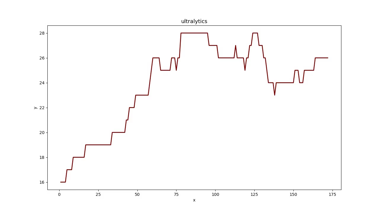 | 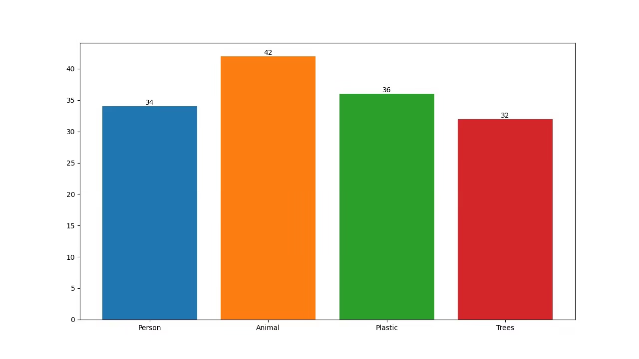 | 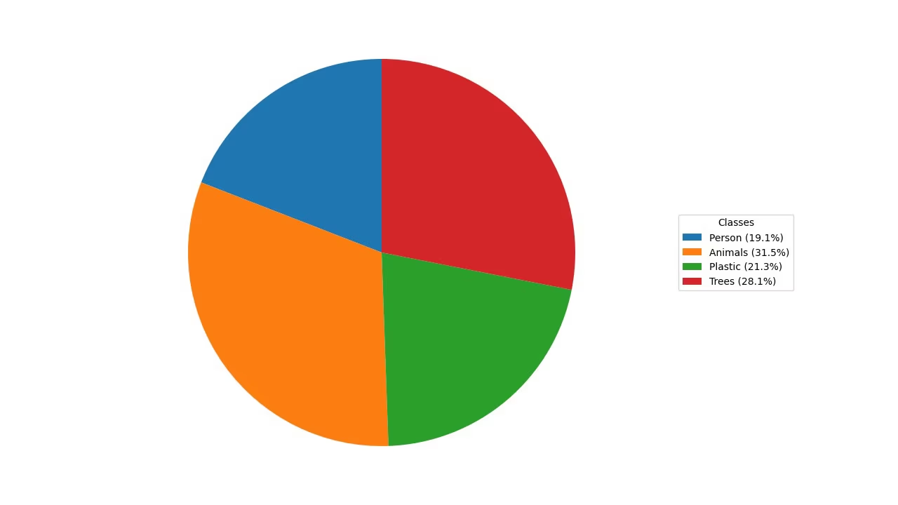 |
Perché visualizzare i dati di rilevamento?#
- I grafici a linee sono ideali per monitorare le variazioni su periodi brevi e lunghi e per confrontare l'andamento di più gruppi nello stesso periodo.
- I grafici a barre sono adatti per confrontare quantità tra categorie diverse e mostrare le relazioni tra una categoria e il suo valore numerico.
- I grafici a torta sono efficaci per illustrare le proporzioni tra categorie e mostrare le parti di un insieme.
- I grafici ad area riempiono lo spazio sotto il grafico a linee, rendendo più immediata la lettura dei conteggi degli oggetti per classe nel tempo.
Genera grafici di analisi#
Passa il video alla soluzione Analytics e seleziona un grafico con analytics_type. La soluzione esegue il rilevamento e il tracciamento su ogni fotogramma e disegna un grafico da 1280×720 (per impostazione predefinita), che puoi scrivere direttamente in un video di output. Passa da "line" a "bar", "pie" e "area" con un solo argomento.
yolo solutions analytics show=True

# Pass the source
yolo solutions analytics source="path/to/video.mp4"

# Generate the pie chart
yolo solutions analytics analytics_type="pie" show=True

# Generate the bar plots
yolo solutions analytics analytics_type="bar" show=True

# Generate the area plots
yolo solutions analytics analytics_type="area" show=True
Argomenti di Analytics#
Ecco una tabella che riepiloga gli argomenti di Analytics:
| Argomento | Tipo | Predefinito | Descrizione |
|---|---|---|---|
model | str | None | Percorso a un file modello Ultralytics YOLO. |
analytics_type | str | 'line' | Tipo di grafico, ad es. line, bar, area o pie. |
figsize | tuple[float, float] | (12.8, 7.2) | Dimensioni della figura in pollici per i grafici Analytics; (12.8, 7.2) genera un fotogramma da 1280×720. |
line_width | int | 2 | Spessore delle linee dei riquadri, dei punti chiave e dei conteggi disegnati dalla soluzione. |
verbose | bool | True | Abilita il log per frame della soluzione, con forma dell'input, conteggi per classe e velocità di elaborazione. La chiamata di tracking è sempre silenziosa. |
Puoi usare anche gli argomenti track nella soluzione Analytics.
| Argomento | Tipo | Predefinito | Descrizione |
|---|---|---|---|
tracker | str | 'tracktrack.yaml' | Specifica l'algoritmo di tracciamento da usare. Opzioni integrate: botsort.yaml, bytetrack.yaml, ocsort.yaml, deepocsort.yaml, fasttrack.yaml, tracktrack.yaml. |
conf | float | 0.25 | Imposta la soglia di confidenza per le rilevazioni; valori più bassi consentono di tracciare più oggetti, ma possono includere falsi positivi. |
iou | float | 0.5 | Imposta la soglia di Intersezione sull'unione (IoU) per filtrare le rilevazioni sovrapposte. |
classes | list | None | Filtra i risultati in base all'indice della classe. Ad esempio, classes=[0, 2, 3] traccia solo le classi specificate. |
device | str | None | Specifica il dispositivo per l'inferenza (ad es. cpu, cuda:0 o 0). Consente di scegliere tra CPU, una GPU specifica o altri dispositivi di calcolo per l'esecuzione del modello. |
imgsz | int or tuple | 640 | Dimensione dell'immagine di destinazione per l'inferenza: un intero per un'immagine quadrata o una coppia (height, width). Le forme vengono adattate allo stride del modello. |
max_det | int | 300 | Numero massimo di rilevazioni da mantenere per fotogramma prima del tracciamento, che limita gli oggetti elaborati da una soluzione nelle scene dense. |
quantize | int or str | None | Precisione dell’inferenza: 16 (FP16) oppure 32/unset (FP32) per i modelli PyTorch e TorchScript quando non si usa la CPU; gli altri formati usano la precisione selezionata dal rispettivo artefatto e ambiente di esecuzione. Sostituisce l’argomento deprecato half. |
Sono inoltre supportati i seguenti argomenti di visualizzazione:
| Argomento | Tipo | Predefinito | Descrizione |
|---|---|---|---|
show | bool | False | Se True, mostra le immagini o i video annotati in una finestra. Utile per ottenere un riscontro visivo immediato durante lo sviluppo o i test. |
Conclusione#
Capire quando e come usare i diversi tipi di visualizzazione è fondamentale per un'analisi efficace dei dati. I grafici a linee, a barre, a torta e ad area sono strumenti essenziali che possono aiutarti a raccontare i tuoi dati in modo più chiaro ed efficace. La soluzione Analytics di Ultralytics YOLO26 offre un modo semplice per generare queste visualizzazioni dai risultati del rilevamento e del tracciamento degli oggetti, facilitando l'estrazione di informazioni utili dai dati visivi.
Domande frequenti#
Per creare un grafico a linee con Ultralytics YOLO26 Analytics, segui questi passaggi:
- Carica un modello YOLO26 e apri il file video.
- Inizializza la classe
Analyticsconanalytics_type="line". - Scorri i fotogrammi del video, chiamando la soluzione a ogni fotogramma per aggiornare il grafico a linee con dati come i conteggi degli oggetti.
- Scrivi
results.plot_imin un video di output per salvare il grafico.
Usa come punto di partenza l'esempio Python qui sopra: esegue già l'intero ciclo sui fotogrammi e il grafico a linee è il
analytics_typepredefinito.Usare Ultralytics YOLO26 per creare grafici a barre offre diversi vantaggi:
- Visualizzazione dei dati in tempo reale: integra i risultati del rilevamento degli oggetti nei grafici a barre per aggiornarli dinamicamente.
- Facilità d'uso: API e funzioni semplici rendono immediata l'implementazione e la visualizzazione dei dati.
- Personalizzazione: personalizza titoli, etichette, colori e altro per adattarli alle tue esigenze specifiche.
- Efficienza: gestisce efficacemente grandi quantità di dati e aggiorna i grafici in tempo reale durante l'elaborazione dei video.
Per generare un grafico a barre, imposta
analytics_type="bar"nell'esempio Python qui sopra: il resto del ciclo sui fotogrammi è identico. Consulta la sezione Esempi visivi per un'anteprima.Ultralytics YOLO26 è un'ottima scelta per creare grafici a torta perché:
- Integrazione con il rilevamento degli oggetti: integra direttamente i risultati del rilevamento degli oggetti nei grafici a torta per ottenere informazioni immediate.
- API intuitiva: semplice da configurare e usare con poche righe di codice.
- Personalizzabile: offre diverse opzioni di personalizzazione per colori, etichette e altro.
- Aggiornamenti in tempo reale: gestisce e visualizza i dati in tempo reale, una caratteristica ideale per i progetti di analisi video.
Per generare un grafico a torta, imposta
analytics_type="pie"nell'esempio Python qui sopra. Per ulteriori informazioni, consulta la sezione Esempi visivi della guida.Sì. Il tracciamento è integrato nella soluzione
Analytics: traccia più oggetti in tempo reale e aggiorna il grafico ogni 30 fotogrammi usando i dati degli oggetti tracciati, così grafici a linee, a barre, a torta e ad area riflettono tutti i conteggi aggiornati. È proprio ciò che fa il ciclo sui fotogrammi nell'esempio Python qui sopra. Per informazioni sulla funzionalità di tracciamento sottostante, consulta la sezione Tracciamento.Ultralytics YOLO26 si distingue per diversi motivi dalle altre soluzioni di rilevamento degli oggetti, come OpenCV e TensorFlow:
- Precisione all'avanguardia: YOLO26 offre una precisione superiore nelle attività di rilevamento degli oggetti, segmentazione delle istanze, segmentazione semantica e classificazione.
- Facilità d'uso: l'API intuitiva consente un'implementazione e un'integrazione rapide senza dover scrivere molto codice.
- Prestazioni in tempo reale: ottimizzato per inferenze ad alta velocità, è adatto alle applicazioni in tempo reale.
- Ampia varietà di applicazioni: supporta il tracciamento di più oggetti, l'addestramento di modelli personalizzati e l'esportazione in formati diversi come ONNX, TensorRT e CoreML.
- Documentazione completa: ampia documentazione e risorse del blog per guidare gli utenti in ogni fase.


Commenti17
Fai una domanda, condividi i tuoi risultati o aiuta qualcun altro.
 User
Hello @glenn-jocher How we can optimize/modify the code for YOLO predict, so it can also give final compiled result of prediction as graph. In case of counting objects/cells classed as different categories in images stored in a root folder. Not just the images with the prediction boxes.
yolo train model=yolo11n.pt data=coco8.yaml epochs=100 imgsz=640
yolo predict model=yolo11n.pt source=path/to/bus.jpg
Like the count graph YOLO makes after training or bar/pie chart?
Thanks
- User
@pderrenger Greetings
- User
Hello,
In relation to the above question, will this code work?
#!/usr/bin/env python3 """ yolo_predict_results.py
Run YOLO predictions on a single image or a directory of images, save annotated images, export per-image and aggregate counts to CSV, and save plots (aggregate bar chart and optional stacked per-image bar chart).
Requirements: pip install ultralytics pandas matplotlib pillow
Usage (recommended - command line): # Single image python yolo_predict_results.py --model /path/to/yolo11n.pt --source /path/to/bus.jpg --output results --save-annotated --plot-aggregate
# Directory (batch)
python yolo_predict_results.py --model /path/to/yolo11n.pt --source /path/to/images_dir --output results --save-annotated --plot-per-image --plot-aggregate
This file includes clearly highlighted comments showing exactly where to set your model path and images directory if you prefer to hardcode them in the script instead of using CLI args. """
import argparse from collections import Counter from pathlib import Path import sys
import numpy as np import pandas as pd import matplotlib.pyplot as plt from PIL import Image
try: from ultralytics import YOLO except Exception as e: print("Please install ultralytics (pip install ultralytics).") raise
IMAGE_EXTS = {".jpg", ".jpeg", ".png", ".bmp", ".tif", ".tiff", ".webp"}
def find_images(directory: Path): return [str(p) for p in sorted(directory.rglob("*")) if p.suffix.lower() in IMAGE_EXTS]
def predict_images(model, paths, conf=0.25, imgsz=640, device=None, save_annotated=False, out_dir=None): """ Run prediction per-image (keeps mapping simple). Returns list of dicts: {'file': path, 'counts': Counter, 'total': int} """ out_dir = Path(out_dir) if out_dir is not None else None annotated_dir = (out_dir / "annotated") if (save_annotated and out_dir is not None) else None if annotated_dir: annotated_dir.mkdir(parents=True, exist_ok=True)
results = []
for p in paths:
    print(f"Predicting: {p}")
    res_list = model.predict(source=p, conf=conf, imgsz=imgsz, device=device, verbose=False)
    if not res_list:
        print(f"Warning: no result for {p}")
        continue
    r = res_list[0]

    counts = Counter()
    try:
        box_cls = getattr(r.boxes, "cls", None)
        if box_cls is not None:
            try:
                arr = box_cls.cpu().numpy()
            except Exception:
                arr = np.array(box_cls)
            arr = arr.astype(int).flatten()
            for c in arr:
                name = model.names.get(int(c), str(int(c)))
                counts[name] += 1
    except Exception as e:
        print(f"Warning: could not parse classes for {p}: {e}")

    total = sum(counts.values())
    results.append({"file": p, "counts": counts, "total": total})

    if save_annotated and annotated_dir:
        try:
            ann = r.plot()
            if isinstance(ann, np.ndarray):
                img_out = Image.fromarray(ann)
            else:
                img_out = ann
            out_path = annotated_dir / (Path(p).stem + "_annotated" + Path(p).suffix)
            img_out.save(out_path)
        except Exception as e:
            print(f"Warning: failed to save annotated image for {p}: {e}")

return results
def build_dataframe(summary): all_classes = set() for row in summary: all_classes.update(row["counts"].keys()) classes = sorted(all_classes)
rows = []
for row in summary:
    data = {cls: row["counts"].get(cls, 0) for cls in classes}
    data["file"] = row["file"]
    data["total"] = row["total"]
    rows.append(data)

if not rows:
    # Return empty dataframe
    df = pd.DataFrame(columns=["file", "total"] + classes)
else:
    df = pd.DataFrame(rows)
    cols = ["file"] + classes + ["total"]
    df = df[cols]
return df, classes
def save_csvs(summary, out_dir: Path): df, classes = build_dataframe(summary) out_dir.mkdir(parents=True, exist_ok=True) csv1 = out_dir / "counts_per_image.csv" df.to_csv(csv1, index=False) print(f"Saved per-image counts to: {csv1}")
agg = Counter()
for r in summary:
    agg.update(r["counts"])
agg_series = pd.Series(dict(agg)).sort_values(ascending=False)
csv2 = out_dir / "aggregate_counts.csv"
agg_series.to_csv(csv2, header=["count"])
print(f"Saved aggregate counts to: {csv2}")
return df, classes, agg
def plot_aggregate(agg_counter, out_path: Path): names = list(agg_counter.keys()) counts = [agg_counter[n] for n in names] fig, ax = plt.subplots(figsize=(max(6, len(names) * 0.6), 5)) ax.bar(names, counts, color="tab:blue") ax.set_ylabel("Count") ax.set_title("Aggregate object counts") plt.xticks(rotation=45, ha="right") plt.tight_layout() out_path.parent.mkdir(parents=True, exist_ok=True) fig.savefig(out_path) plt.close(fig) print(f"Saved aggregate plot to: {out_path}")
def plot_stacked_per_image(df: pd.DataFrame, classes, out_path: Path, top_n=50): if df.empty: print("No per-image data to plot.") return plot_df = df.copy() if top_n and len(plot_df) > top_n: plot_df = plot_df.sort_values("total", ascending=False).head(top_n) x = plot_df["file"].apply(lambda p: Path(p).name).tolist() bottoms = np.zeros(len(plot_df)) fig, ax = plt.subplots(figsize=(max(8, len(x) * 0.6), 6)) for cls in classes: vals = plot_df[cls].values ax.bar(x, vals, bottom=bottoms, label=cls) bottoms += vals ax.set_ylabel("Counts") ax.set_title("Per-image stacked counts") ax.legend(bbox_to_anchor=(1.05, 1), loc="upper left") plt.xticks(rotation=45, ha="right") plt.tight_layout() out_path.parent.mkdir(parents=True, exist_ok=True) fig.savefig(out_path) plt.close(fig) print(f"Saved per-image stacked plot to: {out_path}")
def main(): ap = argparse.ArgumentParser(description="YOLO predict -> save CSV + plots") ap.add_argument("--model", required=False, help="Path to YOLO model (.pt) (e.g., yolo11n.pt)") ap.add_argument("--source", required=False, help="Image file or directory of images") ap.add_argument("--output", required=False, help="Output directory", default="results") ap.add_argument("--conf", type=float, default=0.25, help="Confidence threshold") ap.add_argument("--imgsz", type=int, default=640, help="Image size for inference") ap.add_argument("--device", type=str, default=None, help="Device (e.g., 0 or 'cpu')") ap.add_argument("--save-annotated", action="store_true", help="Save annotated images") ap.add_argument("--plot-per-image", action="store_true", help="Save stacked per-image plot") ap.add_argument("--plot-aggregate", action="store_true", help="Save aggregate bar chart") ap.add_argument("--top-n", type=int, default=50, help="Top N images for per-image plot when many images")
# Parse CLI args (recommended usage)
args = ap.parse_args()

# -------------------------------------------------------------------------
# HIGHLIGHT 1: If you want to hardcode paths, replace the `args = ap.parse_args()` line
# with the block below. Edit the two highlighted lines inside the block:
#    model="..."   <-- SET YOUR MODEL FILE PATH HERE
#    source="..."  <-- SET YOUR IMAGE FILE OR IMAGES DIRECTORY PATH HERE
#
# Example (UNCOMMENT and EDIT, then COMMENT OUT or REMOVE the args = ap.parse_args() above):
#
# args = argparse.Namespace(
#     model="/path/to/yolo11n.pt",       # <<< HIGHLIGHT: set model path here (absolute or relative)
#     source="/path/to/images_or_image", # <<< HIGHLIGHT: set image file or images directory path here
#     output="results",
#     conf=0.25,
#     imgsz=640,
#     device=None,
#     save_annotated=True,
#     plot_per_image=True,
#     plot_aggregate=True,
#     top_n=50
# )
# -------------------------------------------------------------------------

# -------------------------------------------------------------------------
# HIGHLIGHT 2: If you prefer using the command-line, supply these two args when
# running the script:
#   --model /path/to/yolo11n.pt
#   --source /path/to/images_or_image
# These correspond to the variables used below: args.model and args.source
# -------------------------------------------------------------------------

if not args.model or not args.source:
    print("Error: --model and --source are required (or hardcode them in the script).")
    print("Example:")
    print("  python yolo_predict_results.py --model /path/to/yolo11n.pt --source /path/to/images --output results --save-annotated --plot-aggregate")
    sys.exit(1)

model_path = Path(args.model)
source = Path(args.source)
out_dir = Path(args.output)
out_dir.mkdir(parents=True, exist_ok=True)

print(f"Loading model: {model_path}")
model = YOLO(str(model_path))

if source.is_dir():
    files = find_images(source)
    if not files:
        print(f"No images found under {source}")
        sys.exit(1)
elif source.is_file():
    files = [str(source)]
else:
    print(f"Source path not found: {source}")
    sys.exit(1)

summary = predict_images(
    model=model,
    paths=files,
    conf=args.conf,
    imgsz=args.imgsz,
    device=args.device,
    save_annotated=args.save_annotated,
    out_dir=out_dir,
)

if not summary:
    print("No predictions were produced.")
    sys.exit(0)

df, classes, agg = save_csvs(summary, out_dir)

if args.plot_aggregate:
    plot_aggregate(agg, out_dir / "aggregate_counts.png")

if args.plot_per_image:
    plot_stacked_per_image(df, classes, out_dir / "per_image_stacked_counts.png", top_n=args.top_n)

print("All done. Results in:", out_dir.resolve())
if name == "main": main()
 Glenn JocherUltralytics
@MUK003 great question, and thanks for sharing the script in detail.
The short answer is: yes, this is a reasonable way to get per-image and aggregate count graphs from YOLO11 predictions, since
YOLO('yolo11n.pt')returnsResultsobjects wherer.boxes.clsholds the class indices and yourCounter/CSV/Matplotlib logic will work on top of that. I’d recommend first running it on a very small image folder and confirming that the numbers incounts_per_image.csvandaggregate_counts.csvmatch what you expect from a few sample images.From the Ultralytics side there’s currently no built-in
yolo predictCLI flag that directly produces those bar/pie charts like training; your Python approach (or, for video streams, thesolutions.Analyticscharts) is the right pattern. For reference on how analytics is structured inside Ultralytics, you can also glance at the Analytics solution API docs.- User
@glenn-jocher Many thanks :)
yeongnamtan
thank you very much @glenn-jocher
How to integrate the code for line graph with line counter ?
- Glenn JocherUltralytics(modificato)
@yeongnamtan to integrate the line graph with a line counter, use the
Analyticsclass to update the line graph with the total object counts per frame. Ensure you initialize theAnalyticswithanalytics_type="line"and update it within your video processing loop. For detailed guidance, please refer to the analytics section in the documentation.
Peymankar
Hi, how can i count number of left turns or right turns in an intersection?
- Glenn JocherUltralytics
@Peymankar hello!
To count the number of left or right turns at an intersection using Ultralytics YOLO, you can set up a tracking system that identifies and follows each vehicle's trajectory. Here’s a brief outline on how you might approach this:
-
Track Vehicles: Use the YOLO model to detect and track vehicles. You can use the
model.track()function to keep track of each vehicle's movement frame by frame. -
Define Zones: Define areas or lines within the video frame that represent the boundaries of different turn directions (left, right).
-
Analyze Trajectories: Analyze the paths of tracked vehicles to determine when they cross these defined zones. This can be done by checking the intersection of vehicle tracks with these zones and classifying the movement as a left or right turn based on the zone they intersect.
-
Count Turns: Maintain a count of how many vehicles make left or right turns based on these intersections.
For a more detailed guide on setting up vehicle tracking and analyzing trajectories, you might find the tracking and analytics features in the Ultralytics documentation helpful. Implementing this will require some custom coding to define zones and analyze paths relative to these zones.
If you need further assistance or more specific guidance, feel free to ask. Happy coding! 😊
-
ani = FuncAnimation(fig, animate, frames=range(int(cap.get(cv2.CAP_PROP_FRAME_COUNT))), blit=False, interval=1000/fps, repeat=False)
plt.show()
The code is still not working... I
error meesage ... WARNING ⚠️ best.pt appears to require 'dill', which is not in ultralytics requirements. AutoInstall will run now for 'dill' but this feature will be removed in the future. Recommend fixes are to train a new model using the latest 'ultralytics' package or to run a command with an official YOLOv8 model, i.e. 'yolo predict model=yolov8n.pt' requirements: Ultralytics requirement ['dill'] not found, attempting AutoUpdate... Collecting dill Downloading dill-0.3.8-py3-none-any.whl (116 kB) ━━━━━━━━━━━━━━━━━━━━━━━━━━━━━━━━━━━━━━━━ 116.3/116.3 kB 4.9 MB/s eta 0:00:00 Installing collected packages: dill Successfully installed dill-0.3.8
requirements: AutoUpdate success ✅ 5.8s, installed 1 package: ['dill'] requirements: ⚠️ Restart runtime or rerun command for updates to take effect
requirements: Ultralytics requirement ['lapx>=0.5.2'] not found, attempting AutoUpdate... Collecting lapx>=0.5.2 Downloading lapx-0.5.9-cp310-cp310-manylinux_2_5_x86_64.manylinux1_x86_64.manylinux_2_17_x86_64.manylinux2014_x86_64.whl (1.7 MB) ━━━━━━━━━━━━━━━━━━━━━━━━━━━━━━━━━━━━━━━━ 1.7/1.7 MB 11.8 MB/s eta 0:00:00 Requirement already satisfied: numpy>=1.21.6 in /usr/local/lib/python3.10/dist-packages (from lapx>=0.5.2) (1.25.2) Installing collected packages: lapx Successfully installed lapx-0.5.9
requirements: AutoUpdate success ✅ 7.4s, installed 1 package: ['lapx>=0.5.2'] requirements: ⚠️ Restart runtime or rerun command for updates to take effect
0: 384x640 2 fishs, 134.7ms Speed: 13.4ms preprocess, 134.7ms inference, 747.7ms postprocess per image at shape (1, 3, 384, 640)
DisabledFunctionError Traceback (most recent call last) in <cell line: 26>() 37 clswise_count[model.names[int(cls)]] = 1 38 ---> 39 analytics.update_bar(clswise_count) 40 cv2_imshow('Bar Plot', frame) 41 clswise_count = {}
1 frames /usr/local/lib/python3.10/dist-packages/google/colab/_import_hooks/_cv2.py in wrapped(*args, **kwargs) 46 def wrapped(*args, **kwargs): 47 if not os.environ.get(env_var, False): ---> 48 raise DisabledFunctionError(message, name or func.name) 49 return func(*args, **kwargs) 50
DisabledFunctionError: cv2.imshow() is disabled in Colab, because it causes Jupyter sessions to crash; see https://github.com/jupyter/notebook/issues/3935. As a substitution, consider using from google.colab.patches import cv2_imshow
 Paula DerrengerUltralytics
Hello,
Thank you for sharing the details of the issue you're encountering. It seems like the
dillandlapxpackages were missing but have now been successfully installed. Please ensure you restart your runtime or rerun your command to allow the updates to take effect, as suggested by the AutoUpdate messages.Regarding the
DisabledFunctionErrorforcv2.imshow()in Colab, this function is indeed disabled because it can cause Jupyter sessions to crash. As an alternative, you can usecv2_imshowfrom thegoogle.colab.patchesmodule to display images in Colab notebooks. Here’s how you can modify your code:from google.colab.patches import cv2_imshow # Replace cv2.imshow with cv2_imshow cv2_imshow(frame)This should allow you to display images without causing any issues in your Colab environment.
If you have any more questions or need further assistance, feel free to ask. Happy coding! 🚀
thank you
In the code for bar plots , I don't see any cv2.imshow. when I run the code, I get cv2.imshow error.
- Paula DerrengerUltralytics
@yeongnamtan hello,
It seems like you're encountering an issue with
cv2.imshownot being present in the bar plot code example. This function is indeed necessary to display the frames with the visualizations in real-time. To resolve the error, you can add the following line just after updating the bar plot in the loop:cv2.imshow('Bar Plot', frame)Make sure to include this inside the loop where frames are being processed, and it will display the updated frame with the bar plot. Additionally, ensure that you have the line
if cv2.waitKey(1) & 0xFF == ord('q'):to handle the window closure properly.If you need further assistance or have more questions, feel free to ask!
I tried to use google colab but it is giving me error because of cv2.imshow... How can I modify it to use cv2_imshow instead ... from google.colab.patches import cv2_imshow # Import cv2_imshow from google.colab.patches
DisabledFunctionError: cv2.imshow() is disabled in Colab, because it causes Jupyter sessions to crash; see https://github.com/jupyter/notebook/issues/3935. As a substitution, consider using from google.colab.patches import cv2_imshow
- Paula DerrengerUltralytics
Hello! To use
cv2_imshowinstead ofcv2.imshowin Google Colab, you can make a simple modification to your code. First, ensure you importcv2_imshowfromgoogle.colab.patchesas you've mentioned. Then, replace all instances ofcv2.imshowwithcv2_imshow. Here’s how you can do it:-
Import the function:
from google.colab.patches import cv2_imshow -
Replace
cv2.imshowwithcv2_imshow:# Instead of cv2.imshow("Frame", frame) cv2_imshow(frame)
This change should resolve the issue with displaying images in Google Colab. Let me know if there's anything else you need help with! 😊
-