YOLOv7: Trainable Bag-of-Freebies

YOLOv7 is a state-of-the-art real-time object detector that surpasses all known object detectors in both speed and accuracy in the range from 5 FPS to 160 FPS. It has the highest accuracy (56.8% AP) among all known real-time object detectors with 30 FPS or higher on GPU V100. Moreover, YOLOv7 outperforms other object detectors such as YOLOR, YOLOX, Scaled-YOLOv4, YOLOv5, and many others in speed and accuracy. The model is trained on the MS COCO dataset from scratch without using any other datasets or pre-trained weights. Source code for YOLOv7 is available on GitHub.

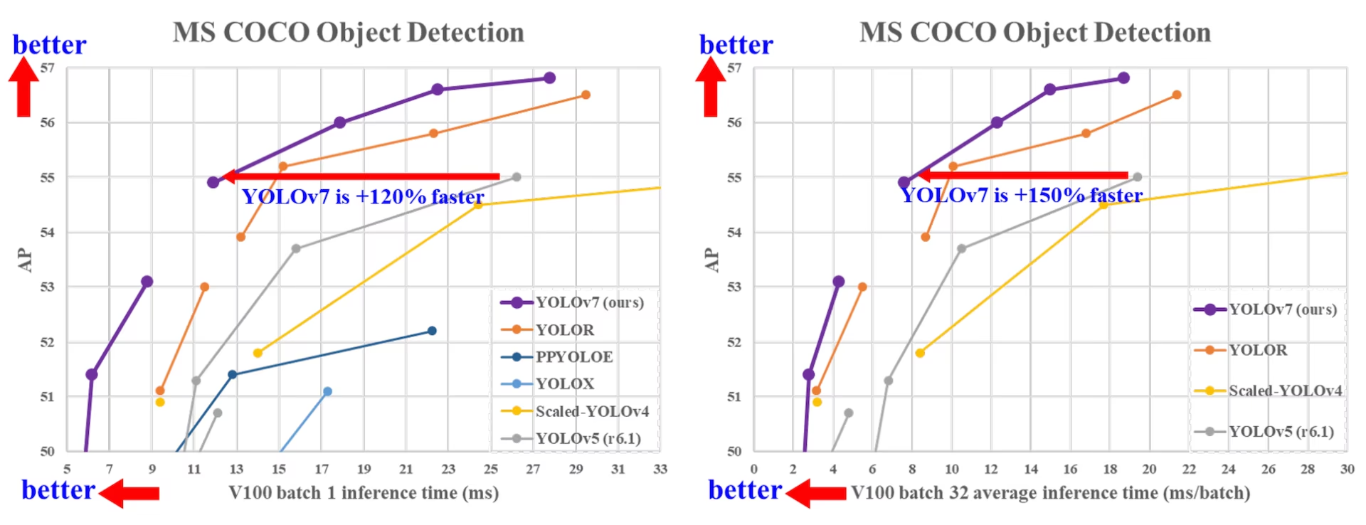
Comparison of SOTA object detectors

From the results in the YOLO comparison table we know that the proposed method has the best speed-accuracy trade-off comprehensively. If we compare YOLOv7-tiny-SiLU with YOLOv5-N (r6.1), our method is 127 fps faster and 10.7% more accurate on AP. In addition, YOLOv7 has 51.4% AP at frame rate of 161 fps, while PPYOLOE-L with the same AP has only 78 fps frame rate. In terms of parameter usage, YOLOv7 is 41% less than PPYOLOE-L. If we compare YOLOv7-X with 114 fps inference speed to YOLOv5-L (r6.1) with 99 fps inference speed, YOLOv7-X can improve AP by 3.9%. If YOLOv7-X is compared with YOLOv5-X (r6.1) of similar scale, the inference speed of YOLOv7-X is 31 fps faster. In addition, in terms the amount of parameters and computation, YOLOv7-X reduces 22% of parameters and 8% of computation compared to YOLOv5-X (r6.1), but improves AP by 2.2% (Source).

Overview

Real-time object detection is an important component in many computer vision systems, including multi-object tracking, autonomous driving, robotics, and medical image analysis. In recent years, real-time object detection development has focused on designing efficient architectures and improving the inference speed of various CPUs, GPUs, and neural processing units (NPUs). YOLOv7 supports both mobile GPU and GPU devices, from the edge to the cloud.

Unlike traditional real-time object detectors that focus on architecture optimization, YOLOv7 introduces a focus on the optimization of the training process. This includes modules and optimization methods designed to improve the accuracy of object detection without increasing the inference cost, a concept known as the "trainable bag-of-freebies".

Key Features

YOLOv7 introduces several key features:

1. Model Re-parameterization: YOLOv7 proposes a planned re-parameterized model, which is a strategy applicable to layers in different networks with the concept of gradient propagation path.

2. Dynamic Label Assignment: The training of the model with multiple output layers presents a new issue: "How to assign dynamic targets for the outputs of different branches?" To solve this problem, YOLOv7 introduces a new label assignment method called coarse-to-fine lead guided label assignment.

3. Extended and Compound Scaling: YOLOv7 proposes "extend" and "compound scaling" methods for the real-time object detector that can effectively utilize parameters and computation.

4. Efficiency: The method proposed by YOLOv7 can effectively reduce about 40% parameters and 50% computation of state-of-the-art real-time object detector, and has faster inference speed and higher detection accuracy.

Usage Examples

As of the time of writing, Ultralytics does not currently support YOLOv7 models. Therefore, any users interested in using YOLOv7 will need to refer directly to the YOLOv7 GitHub repository for installation and usage instructions.

Here is a brief overview of the typical steps you might take to use YOLOv7:

1. Visit the YOLOv7 GitHub repository: https://github.com/WongKinYiu/yolov7.

2. Follow the instructions provided in the README file for installation. This typically involves cloning the repository, installing necessary dependencies, and setting up any necessary environment variables.

3. Once installation is complete, you can train and use the model as per the usage instructions provided in the repository. This usually involves preparing your dataset, configuring the model parameters, training the model, and then using the trained model to perform object detection.

Please note that the specific steps may vary depending on your specific use case and the current state of the YOLOv7 repository. Therefore, it is strongly recommended to refer directly to the instructions provided in the YOLOv7 GitHub repository.

We regret any inconvenience this may cause and will strive to update this document with usage examples for Ultralytics once support for YOLOv7 is implemented.

Citations and Acknowledgements

We would like to acknowledge the YOLOv7 authors for their significant contributions in the field of real-time object detection:

@article{wang2022yolov7,
  title={{YOLOv7}: Trainable bag-of-freebies sets new state-of-the-art for real-time object detectors},
  author={Wang, Chien-Yao and Bochkovskiy, Alexey and Liao, Hong-Yuan Mark},
  journal={arXiv preprint arXiv:2207.02696},
  year={2022}
}

The original YOLOv7 paper can be found on arXiv. The authors have made their work publicly available, and the codebase can be accessed on GitHub. We appreciate their efforts in advancing the field and making their work accessible to the broader community.

FAQ

What is YOLOv7 and why is it considered a breakthrough in real-time object detection?

YOLOv7 is a cutting-edge real-time object detection model that achieves unparalleled speed and accuracy. It surpasses other models, such as YOLOX, YOLOv5, and PPYOLOE, in both parameters usage and inference speed. YOLOv7's distinguishing features include its model re-parameterization and dynamic label assignment, which optimize its performance without increasing inference costs. For more technical details about its architecture and comparison metrics with other state-of-the-art object detectors, refer to the YOLOv7 paper.

How does YOLOv7 improve on previous YOLO models like YOLOv4 and YOLOv5?

YOLOv7 introduces several innovations, including model re-parameterization and dynamic label assignment, which enhance the training process and improve inference accuracy. Compared to YOLOv5, YOLOv7 significantly boosts speed and accuracy. For instance, YOLOv7-X improves accuracy by 2.2% and reduces parameters by 22% compared to YOLOv5-X. Detailed comparisons can be found in the performance table YOLOv7 comparison with SOTA object detectors.

Can I use YOLOv7 with Ultralytics tools and platforms?

As of now, Ultralytics does not directly support YOLOv7 in its tools and platforms. Users interested in using YOLOv7 need to follow the installation and usage instructions provided in the YOLOv7 GitHub repository. For other state-of-the-art models, you can explore and train using Ultralytics tools like Ultralytics HUB.

How do I install and run YOLOv7 for a custom object detection project?

To install and run YOLOv7, follow these steps:

1. Clone the YOLOv7 repository:

   git clone https://github.com/WongKinYiu/yolov7
   

2. Navigate to the cloned directory and install dependencies:

   cd yolov7
   pip install -r requirements.txt
   

3. Prepare your dataset and configure the model parameters according to the usage instructions provided in the repository. For further guidance, visit the YOLOv7 GitHub repository for the latest information and updates.

What are the key features and optimizations introduced in YOLOv7?

YOLOv7 offers several key features that revolutionize real-time object detection:

• Model Re-parameterization: Enhances the model's performance by optimizing gradient propagation paths.
• Dynamic Label Assignment: Uses a coarse-to-fine lead guided method to assign dynamic targets for outputs across different branches, improving accuracy.
• Extended and Compound Scaling: Efficiently utilizes parameters and computation to scale the model for various real-time applications.
• Efficiency: Reduces parameter count by 40% and computation by 50% compared to other state-of-the-art models while achieving faster inference speeds. For further details on these features, see the YOLOv7 Overview section.

Comments