Análisis con Ultralytics YOLO26
El análisis con Ultralytics YOLO26 convierte los resultados de la detección de objetos y el seguimiento en gráficos en tiempo real, para que puedas ver cómo cambian los recuentos de objetos fotograma a fotograma en un vídeo. Esta guía explica cuatro tipos de visualización de datos: gráficos de líneas, gráficos de barras, gráficos circulares y gráficos de áreas, y muestra cómo alternar entre ellos con ejemplos compartidos de Python y CLI.
Ver: Cómo generar gráficos analíticos con Ultralytics | Gráficos de líneas, de barras, de áreas y circulares
Ejemplos visuales#
| Gráfico de líneas | Gráfico de barras | Gráfico circular |
|---|---|---|
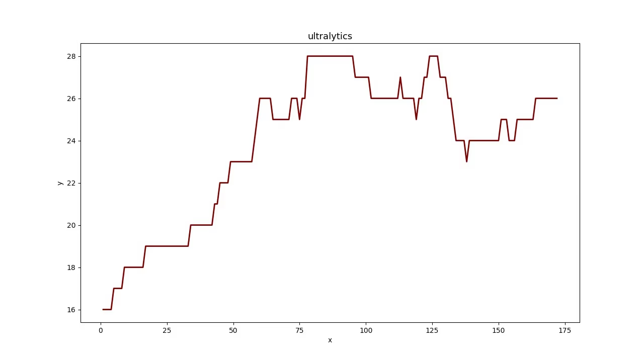 | 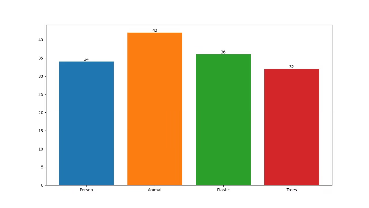 | 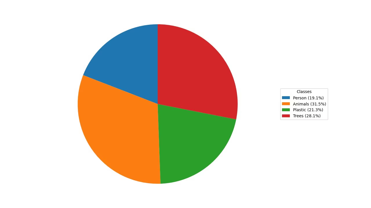 |
¿Por qué visualizar los datos de detección?#
- Los gráficos de líneas son ideales para seguir los cambios durante periodos cortos y largos, así como para comparar los cambios de varios grupos en un mismo periodo.
- Los gráficos de barras son adecuados para comparar cantidades de distintas categorías y mostrar la relación entre una categoría y su valor numérico.
- Los gráficos circulares son eficaces para ilustrar las proporciones entre categorías y mostrar las partes de un conjunto.
- Los gráficos de áreas rellenan el espacio bajo la línea para que los recuentos de objetos por clase a lo largo del tiempo se puedan consultar de un vistazo.
Generar gráficos de análisis#
Pasa el vídeo a la solución Analytics y selecciona un gráfico con analytics_type. La solución ejecuta la detección y el seguimiento en cada fotograma y genera un gráfico de 1280×720 (de forma predeterminada) que puedes escribir directamente en un vídeo de salida. Alterna entre "line", "bar", "pie" y "area" con un solo argumento.
yolo solutions analytics show=True

# Pass the source
yolo solutions analytics source="path/to/video.mp4"

# Generate the pie chart
yolo solutions analytics analytics_type="pie" show=True

# Generate the bar plots
yolo solutions analytics analytics_type="bar" show=True

# Generate the area plots
yolo solutions analytics analytics_type="area" show=True
Argumentos de Analytics#
Esta tabla resume los argumentos de Analytics:
| Argumento | Tipo | Predeterminado | Descripción |
|---|---|---|---|
model | str | None | Ruta a un archivo de modelo Ultralytics YOLO. |
analytics_type | str | 'line' | Tipo de gráfico, es decir, line, bar, area o pie. |
figsize | tuple[float, float] | (12.8, 7.2) | Tamaño de las figuras en pulgadas para los gráficos de Analytics; (12.8, 7.2) genera un fotograma de 1280×720. |
line_width | int | 2 | Grosor de línea de los cuadros, puntos clave y recuentos que dibuja la solución. |
verbose | bool | True | Activa el registro por fotograma de la forma de entrada, los recuentos por clase y la velocidad de procesamiento de la solución. La llamada de seguimiento en sí siempre es silenciosa. |
También puedes utilizar los argumentos de track en la solución Analytics.
| Argumento | Tipo | Predeterminado | Descripción |
|---|---|---|---|
tracker | str | 'tracktrack.yaml' | Especifica el algoritmo de seguimiento que se va a usar. Opciones integradas: botsort.yaml, bytetrack.yaml, ocsort.yaml, deepocsort.yaml, fasttrack.yaml, tracktrack.yaml. |
conf | float | 0.25 | Establece el umbral de confianza de las detecciones; los valores más bajos permiten seguir más objetos, pero pueden incluir falsos positivos. |
iou | float | 0.5 | Establece el umbral de intersección sobre unión (IoU) para filtrar las detecciones solapadas. |
classes | list | None | Filtra los resultados por índice de clase. Por ejemplo, classes=[0, 2, 3] solo sigue las clases especificadas. |
device | str | None | Especifica el dispositivo para la inferencia (p. ej., cpu, cuda:0 o 0). Permite elegir entre CPU, una GPU concreta u otros dispositivos de cálculo para ejecutar el modelo. |
imgsz | int or tuple | 640 | Tamaño de imagen de destino para la inferencia: un entero para una imagen cuadrada o una pareja (height, width). Las dimensiones se ajustan al stride del modelo. |
max_det | int | 300 | Número máximo de detecciones que se conservan por fotograma antes del seguimiento, lo que limita los objetos que procesa una solución en escenas densas. |
quantize | int or str | None | Precisión de inferencia: 16 (FP16) o 32/unset (FP32) para los modelos PyTorch y TorchScript fuera de CPU; los demás formatos usan la precisión que seleccionen el artefacto y el entorno de ejecución. Sustituye al argumento obsoleto half. |
Además, se admiten los siguientes argumentos de visualización:
| Argumento | Tipo | Predeterminado | Descripción |
|---|---|---|---|
show | bool | False | Si True, muestra las imágenes o los vídeos anotados en una ventana. Es útil para obtener información visual inmediata durante el desarrollo o las pruebas. |
Conclusión#
Comprender cuándo y cómo utilizar distintos tipos de visualizaciones es fundamental para analizar datos de forma eficaz. Los gráficos de líneas, los gráficos de barras, los gráficos circulares y los gráficos de áreas son herramientas fundamentales que pueden ayudarte a comunicar la historia que cuentan tus datos con mayor claridad y eficacia. La solución Analytics de Ultralytics YOLO26 ofrece una forma sencilla de generar estas visualizaciones a partir de los resultados de detección y seguimiento de objetos, lo que facilita la extracción de información relevante de tus datos visuales.
Preguntas frecuentes#
Para crear un gráfico de líneas con Ultralytics YOLO26 Analytics, sigue estos pasos:
- Carga un modelo YOLO26 y abre el archivo de vídeo.
- Inicializa la clase
Analyticsconanalytics_type="line". - Recorre los fotogramas del vídeo y llama a la solución en cada uno para actualizar el gráfico de líneas con datos como los recuentos de objetos.
- Escribe
results.plot_imen un vídeo de salida para guardar el gráfico.
Usa el ejemplo de Python anterior como punto de partida: ya incluye el procesamiento de todos los fotogramas, y el gráfico de líneas es el
analytics_typepredeterminado.Usar Ultralytics YOLO26 para crear gráficos de barras ofrece varias ventajas:
- Visualización de datos en tiempo real: Integra los resultados de detección de objetos en gráficos de barras para actualizarlos dinámicamente.
- Facilidad de uso: su API y sus funciones sencillas facilitan la implementación y la visualización de datos.
- Personalización: personaliza títulos, etiquetas, colores y mucho más según tus necesidades.
- Eficiencia: Gestiona grandes volúmenes de datos de forma eficiente y actualiza los gráficos en tiempo real durante el procesamiento de vídeo.
Para generar un gráfico de barras, configura
analytics_type="bar"en el ejemplo de Python anterior; el resto del procesamiento de fotogramas es idéntico. Consulta la sección Ejemplos visuales para ver una muestra.Ultralytics YOLO26 es una opción excelente para crear gráficos circulares porque:
- Integración con la detección de objetos: integra directamente los resultados de la detección de objetos en gráficos circulares para obtener información al instante.
- API fácil de usar: es sencilla de configurar y utilizar, y requiere muy poco código.
- Personalizable: ofrece varias opciones para personalizar los colores, las etiquetas y mucho más.
- Actualizaciones en tiempo real: Gestiona y visualiza datos en tiempo real, una opción ideal para proyectos de análisis de vídeo.
Para generar un gráfico circular, configura
analytics_type="pie"en el ejemplo de Python anterior. Para obtener más información, consulta la sección Ejemplos visuales de la guía.Sí. El seguimiento está integrado en la solución
Analytics: sigue varios objetos en tiempo real y actualiza el gráfico con los datos de los objetos seguidos cada 30 fotogramas, de modo que los gráficos de líneas, barras, circulares y de áreas reflejan los recuentos en directo. Esto es exactamente lo que hace el procesamiento de fotogramas del ejemplo de Python anterior. Para obtener más información sobre la funcionalidad de seguimiento subyacente, consulta la sección Seguimiento.Ultralytics YOLO26 destaca frente a otras soluciones de detección de objetos como OpenCV y TensorFlow por varios motivos:
- Precisión de vanguardia: YOLO26 ofrece una precisión superior en tareas de detección de objetos, segmentación de instancias, segmentación semántica y clasificación.
- Facilidad de uso: su API intuitiva permite implementar e integrar soluciones rápidamente, sin necesidad de programar demasiado.
- Rendimiento en tiempo real: está optimizado para realizar inferencias a gran velocidad, por lo que es adecuado para aplicaciones en tiempo real.
- Diversidad de aplicaciones: admite el seguimiento de varios objetos, el entrenamiento de modelos personalizados y la exportación a distintos formatos, como ONNX, TensorRT y CoreML.
- Documentación completa: cuenta con una amplia documentación y recursos del blog para guiarte en cada paso.


Comentarios17
Haz una pregunta, comparte tus resultados o ayuda a otra persona.
 User
Hello @glenn-jocher How we can optimize/modify the code for YOLO predict, so it can also give final compiled result of prediction as graph. In case of counting objects/cells classed as different categories in images stored in a root folder. Not just the images with the prediction boxes.
yolo train model=yolo11n.pt data=coco8.yaml epochs=100 imgsz=640
yolo predict model=yolo11n.pt source=path/to/bus.jpg
Like the count graph YOLO makes after training or bar/pie chart?
Thanks
- User
@pderrenger Greetings
- User
Hello,
In relation to the above question, will this code work?
#!/usr/bin/env python3 """ yolo_predict_results.py
Run YOLO predictions on a single image or a directory of images, save annotated images, export per-image and aggregate counts to CSV, and save plots (aggregate bar chart and optional stacked per-image bar chart).
Requirements: pip install ultralytics pandas matplotlib pillow
Usage (recommended - command line): # Single image python yolo_predict_results.py --model /path/to/yolo11n.pt --source /path/to/bus.jpg --output results --save-annotated --plot-aggregate
# Directory (batch)
python yolo_predict_results.py --model /path/to/yolo11n.pt --source /path/to/images_dir --output results --save-annotated --plot-per-image --plot-aggregate
This file includes clearly highlighted comments showing exactly where to set your model path and images directory if you prefer to hardcode them in the script instead of using CLI args. """
import argparse from collections import Counter from pathlib import Path import sys
import numpy as np import pandas as pd import matplotlib.pyplot as plt from PIL import Image
try: from ultralytics import YOLO except Exception as e: print("Please install ultralytics (pip install ultralytics).") raise
IMAGE_EXTS = {".jpg", ".jpeg", ".png", ".bmp", ".tif", ".tiff", ".webp"}
def find_images(directory: Path): return [str(p) for p in sorted(directory.rglob("*")) if p.suffix.lower() in IMAGE_EXTS]
def predict_images(model, paths, conf=0.25, imgsz=640, device=None, save_annotated=False, out_dir=None): """ Run prediction per-image (keeps mapping simple). Returns list of dicts: {'file': path, 'counts': Counter, 'total': int} """ out_dir = Path(out_dir) if out_dir is not None else None annotated_dir = (out_dir / "annotated") if (save_annotated and out_dir is not None) else None if annotated_dir: annotated_dir.mkdir(parents=True, exist_ok=True)
results = []
for p in paths:
    print(f"Predicting: {p}")
    res_list = model.predict(source=p, conf=conf, imgsz=imgsz, device=device, verbose=False)
    if not res_list:
        print(f"Warning: no result for {p}")
        continue
    r = res_list[0]

    counts = Counter()
    try:
        box_cls = getattr(r.boxes, "cls", None)
        if box_cls is not None:
            try:
                arr = box_cls.cpu().numpy()
            except Exception:
                arr = np.array(box_cls)
            arr = arr.astype(int).flatten()
            for c in arr:
                name = model.names.get(int(c), str(int(c)))
                counts[name] += 1
    except Exception as e:
        print(f"Warning: could not parse classes for {p}: {e}")

    total = sum(counts.values())
    results.append({"file": p, "counts": counts, "total": total})

    if save_annotated and annotated_dir:
        try:
            ann = r.plot()
            if isinstance(ann, np.ndarray):
                img_out = Image.fromarray(ann)
            else:
                img_out = ann
            out_path = annotated_dir / (Path(p).stem + "_annotated" + Path(p).suffix)
            img_out.save(out_path)
        except Exception as e:
            print(f"Warning: failed to save annotated image for {p}: {e}")

return results
def build_dataframe(summary): all_classes = set() for row in summary: all_classes.update(row["counts"].keys()) classes = sorted(all_classes)
rows = []
for row in summary:
    data = {cls: row["counts"].get(cls, 0) for cls in classes}
    data["file"] = row["file"]
    data["total"] = row["total"]
    rows.append(data)

if not rows:
    # Return empty dataframe
    df = pd.DataFrame(columns=["file", "total"] + classes)
else:
    df = pd.DataFrame(rows)
    cols = ["file"] + classes + ["total"]
    df = df[cols]
return df, classes
def save_csvs(summary, out_dir: Path): df, classes = build_dataframe(summary) out_dir.mkdir(parents=True, exist_ok=True) csv1 = out_dir / "counts_per_image.csv" df.to_csv(csv1, index=False) print(f"Saved per-image counts to: {csv1}")
agg = Counter()
for r in summary:
    agg.update(r["counts"])
agg_series = pd.Series(dict(agg)).sort_values(ascending=False)
csv2 = out_dir / "aggregate_counts.csv"
agg_series.to_csv(csv2, header=["count"])
print(f"Saved aggregate counts to: {csv2}")
return df, classes, agg
def plot_aggregate(agg_counter, out_path: Path): names = list(agg_counter.keys()) counts = [agg_counter[n] for n in names] fig, ax = plt.subplots(figsize=(max(6, len(names) * 0.6), 5)) ax.bar(names, counts, color="tab:blue") ax.set_ylabel("Count") ax.set_title("Aggregate object counts") plt.xticks(rotation=45, ha="right") plt.tight_layout() out_path.parent.mkdir(parents=True, exist_ok=True) fig.savefig(out_path) plt.close(fig) print(f"Saved aggregate plot to: {out_path}")
def plot_stacked_per_image(df: pd.DataFrame, classes, out_path: Path, top_n=50): if df.empty: print("No per-image data to plot.") return plot_df = df.copy() if top_n and len(plot_df) > top_n: plot_df = plot_df.sort_values("total", ascending=False).head(top_n) x = plot_df["file"].apply(lambda p: Path(p).name).tolist() bottoms = np.zeros(len(plot_df)) fig, ax = plt.subplots(figsize=(max(8, len(x) * 0.6), 6)) for cls in classes: vals = plot_df[cls].values ax.bar(x, vals, bottom=bottoms, label=cls) bottoms += vals ax.set_ylabel("Counts") ax.set_title("Per-image stacked counts") ax.legend(bbox_to_anchor=(1.05, 1), loc="upper left") plt.xticks(rotation=45, ha="right") plt.tight_layout() out_path.parent.mkdir(parents=True, exist_ok=True) fig.savefig(out_path) plt.close(fig) print(f"Saved per-image stacked plot to: {out_path}")
def main(): ap = argparse.ArgumentParser(description="YOLO predict -> save CSV + plots") ap.add_argument("--model", required=False, help="Path to YOLO model (.pt) (e.g., yolo11n.pt)") ap.add_argument("--source", required=False, help="Image file or directory of images") ap.add_argument("--output", required=False, help="Output directory", default="results") ap.add_argument("--conf", type=float, default=0.25, help="Confidence threshold") ap.add_argument("--imgsz", type=int, default=640, help="Image size for inference") ap.add_argument("--device", type=str, default=None, help="Device (e.g., 0 or 'cpu')") ap.add_argument("--save-annotated", action="store_true", help="Save annotated images") ap.add_argument("--plot-per-image", action="store_true", help="Save stacked per-image plot") ap.add_argument("--plot-aggregate", action="store_true", help="Save aggregate bar chart") ap.add_argument("--top-n", type=int, default=50, help="Top N images for per-image plot when many images")
# Parse CLI args (recommended usage)
args = ap.parse_args()

# -------------------------------------------------------------------------
# HIGHLIGHT 1: If you want to hardcode paths, replace the `args = ap.parse_args()` line
# with the block below. Edit the two highlighted lines inside the block:
#    model="..."   <-- SET YOUR MODEL FILE PATH HERE
#    source="..."  <-- SET YOUR IMAGE FILE OR IMAGES DIRECTORY PATH HERE
#
# Example (UNCOMMENT and EDIT, then COMMENT OUT or REMOVE the args = ap.parse_args() above):
#
# args = argparse.Namespace(
#     model="/path/to/yolo11n.pt",       # <<< HIGHLIGHT: set model path here (absolute or relative)
#     source="/path/to/images_or_image", # <<< HIGHLIGHT: set image file or images directory path here
#     output="results",
#     conf=0.25,
#     imgsz=640,
#     device=None,
#     save_annotated=True,
#     plot_per_image=True,
#     plot_aggregate=True,
#     top_n=50
# )
# -------------------------------------------------------------------------

# -------------------------------------------------------------------------
# HIGHLIGHT 2: If you prefer using the command-line, supply these two args when
# running the script:
#   --model /path/to/yolo11n.pt
#   --source /path/to/images_or_image
# These correspond to the variables used below: args.model and args.source
# -------------------------------------------------------------------------

if not args.model or not args.source:
    print("Error: --model and --source are required (or hardcode them in the script).")
    print("Example:")
    print("  python yolo_predict_results.py --model /path/to/yolo11n.pt --source /path/to/images --output results --save-annotated --plot-aggregate")
    sys.exit(1)

model_path = Path(args.model)
source = Path(args.source)
out_dir = Path(args.output)
out_dir.mkdir(parents=True, exist_ok=True)

print(f"Loading model: {model_path}")
model = YOLO(str(model_path))

if source.is_dir():
    files = find_images(source)
    if not files:
        print(f"No images found under {source}")
        sys.exit(1)
elif source.is_file():
    files = [str(source)]
else:
    print(f"Source path not found: {source}")
    sys.exit(1)

summary = predict_images(
    model=model,
    paths=files,
    conf=args.conf,
    imgsz=args.imgsz,
    device=args.device,
    save_annotated=args.save_annotated,
    out_dir=out_dir,
)

if not summary:
    print("No predictions were produced.")
    sys.exit(0)

df, classes, agg = save_csvs(summary, out_dir)

if args.plot_aggregate:
    plot_aggregate(agg, out_dir / "aggregate_counts.png")

if args.plot_per_image:
    plot_stacked_per_image(df, classes, out_dir / "per_image_stacked_counts.png", top_n=args.top_n)

print("All done. Results in:", out_dir.resolve())
if name == "main": main()
 Glenn JocherUltralytics
@MUK003 great question, and thanks for sharing the script in detail.
The short answer is: yes, this is a reasonable way to get per-image and aggregate count graphs from YOLO11 predictions, since
YOLO('yolo11n.pt')returnsResultsobjects wherer.boxes.clsholds the class indices and yourCounter/CSV/Matplotlib logic will work on top of that. I’d recommend first running it on a very small image folder and confirming that the numbers incounts_per_image.csvandaggregate_counts.csvmatch what you expect from a few sample images.From the Ultralytics side there’s currently no built-in
yolo predictCLI flag that directly produces those bar/pie charts like training; your Python approach (or, for video streams, thesolutions.Analyticscharts) is the right pattern. For reference on how analytics is structured inside Ultralytics, you can also glance at the Analytics solution API docs.- User
@glenn-jocher Many thanks :)
yeongnamtan
thank you very much @glenn-jocher
How to integrate the code for line graph with line counter ?
- Glenn JocherUltralytics(editado)
@yeongnamtan to integrate the line graph with a line counter, use the
Analyticsclass to update the line graph with the total object counts per frame. Ensure you initialize theAnalyticswithanalytics_type="line"and update it within your video processing loop. For detailed guidance, please refer to the analytics section in the documentation.
Peymankar
Hi, how can i count number of left turns or right turns in an intersection?
- Glenn JocherUltralytics
@Peymankar hello!
To count the number of left or right turns at an intersection using Ultralytics YOLO, you can set up a tracking system that identifies and follows each vehicle's trajectory. Here’s a brief outline on how you might approach this:
-
Track Vehicles: Use the YOLO model to detect and track vehicles. You can use the
model.track()function to keep track of each vehicle's movement frame by frame. -
Define Zones: Define areas or lines within the video frame that represent the boundaries of different turn directions (left, right).
-
Analyze Trajectories: Analyze the paths of tracked vehicles to determine when they cross these defined zones. This can be done by checking the intersection of vehicle tracks with these zones and classifying the movement as a left or right turn based on the zone they intersect.
-
Count Turns: Maintain a count of how many vehicles make left or right turns based on these intersections.
For a more detailed guide on setting up vehicle tracking and analyzing trajectories, you might find the tracking and analytics features in the Ultralytics documentation helpful. Implementing this will require some custom coding to define zones and analyze paths relative to these zones.
If you need further assistance or more specific guidance, feel free to ask. Happy coding! 😊
-
ani = FuncAnimation(fig, animate, frames=range(int(cap.get(cv2.CAP_PROP_FRAME_COUNT))), blit=False, interval=1000/fps, repeat=False)
plt.show()
The code is still not working... I
error meesage ... WARNING ⚠️ best.pt appears to require 'dill', which is not in ultralytics requirements. AutoInstall will run now for 'dill' but this feature will be removed in the future. Recommend fixes are to train a new model using the latest 'ultralytics' package or to run a command with an official YOLOv8 model, i.e. 'yolo predict model=yolov8n.pt' requirements: Ultralytics requirement ['dill'] not found, attempting AutoUpdate... Collecting dill Downloading dill-0.3.8-py3-none-any.whl (116 kB) ━━━━━━━━━━━━━━━━━━━━━━━━━━━━━━━━━━━━━━━━ 116.3/116.3 kB 4.9 MB/s eta 0:00:00 Installing collected packages: dill Successfully installed dill-0.3.8
requirements: AutoUpdate success ✅ 5.8s, installed 1 package: ['dill'] requirements: ⚠️ Restart runtime or rerun command for updates to take effect
requirements: Ultralytics requirement ['lapx>=0.5.2'] not found, attempting AutoUpdate... Collecting lapx>=0.5.2 Downloading lapx-0.5.9-cp310-cp310-manylinux_2_5_x86_64.manylinux1_x86_64.manylinux_2_17_x86_64.manylinux2014_x86_64.whl (1.7 MB) ━━━━━━━━━━━━━━━━━━━━━━━━━━━━━━━━━━━━━━━━ 1.7/1.7 MB 11.8 MB/s eta 0:00:00 Requirement already satisfied: numpy>=1.21.6 in /usr/local/lib/python3.10/dist-packages (from lapx>=0.5.2) (1.25.2) Installing collected packages: lapx Successfully installed lapx-0.5.9
requirements: AutoUpdate success ✅ 7.4s, installed 1 package: ['lapx>=0.5.2'] requirements: ⚠️ Restart runtime or rerun command for updates to take effect
0: 384x640 2 fishs, 134.7ms Speed: 13.4ms preprocess, 134.7ms inference, 747.7ms postprocess per image at shape (1, 3, 384, 640)
DisabledFunctionError Traceback (most recent call last) in <cell line: 26>() 37 clswise_count[model.names[int(cls)]] = 1 38 ---> 39 analytics.update_bar(clswise_count) 40 cv2_imshow('Bar Plot', frame) 41 clswise_count = {}
1 frames /usr/local/lib/python3.10/dist-packages/google/colab/_import_hooks/_cv2.py in wrapped(*args, **kwargs) 46 def wrapped(*args, **kwargs): 47 if not os.environ.get(env_var, False): ---> 48 raise DisabledFunctionError(message, name or func.name) 49 return func(*args, **kwargs) 50
DisabledFunctionError: cv2.imshow() is disabled in Colab, because it causes Jupyter sessions to crash; see https://github.com/jupyter/notebook/issues/3935. As a substitution, consider using from google.colab.patches import cv2_imshow
 Paula DerrengerUltralytics
Hello,
Thank you for sharing the details of the issue you're encountering. It seems like the
dillandlapxpackages were missing but have now been successfully installed. Please ensure you restart your runtime or rerun your command to allow the updates to take effect, as suggested by the AutoUpdate messages.Regarding the
DisabledFunctionErrorforcv2.imshow()in Colab, this function is indeed disabled because it can cause Jupyter sessions to crash. As an alternative, you can usecv2_imshowfrom thegoogle.colab.patchesmodule to display images in Colab notebooks. Here’s how you can modify your code:from google.colab.patches import cv2_imshow # Replace cv2.imshow with cv2_imshow cv2_imshow(frame)This should allow you to display images without causing any issues in your Colab environment.
If you have any more questions or need further assistance, feel free to ask. Happy coding! 🚀
thank you
In the code for bar plots , I don't see any cv2.imshow. when I run the code, I get cv2.imshow error.
- Paula DerrengerUltralytics
@yeongnamtan hello,
It seems like you're encountering an issue with
cv2.imshownot being present in the bar plot code example. This function is indeed necessary to display the frames with the visualizations in real-time. To resolve the error, you can add the following line just after updating the bar plot in the loop:cv2.imshow('Bar Plot', frame)Make sure to include this inside the loop where frames are being processed, and it will display the updated frame with the bar plot. Additionally, ensure that you have the line
if cv2.waitKey(1) & 0xFF == ord('q'):to handle the window closure properly.If you need further assistance or have more questions, feel free to ask!
I tried to use google colab but it is giving me error because of cv2.imshow... How can I modify it to use cv2_imshow instead ... from google.colab.patches import cv2_imshow # Import cv2_imshow from google.colab.patches
DisabledFunctionError: cv2.imshow() is disabled in Colab, because it causes Jupyter sessions to crash; see https://github.com/jupyter/notebook/issues/3935. As a substitution, consider using from google.colab.patches import cv2_imshow
- Paula DerrengerUltralytics
Hello! To use
cv2_imshowinstead ofcv2.imshowin Google Colab, you can make a simple modification to your code. First, ensure you importcv2_imshowfromgoogle.colab.patchesas you've mentioned. Then, replace all instances ofcv2.imshowwithcv2_imshow. Here’s how you can do it:-
Import the function:
from google.colab.patches import cv2_imshow -
Replace
cv2.imshowwithcv2_imshow:# Instead of cv2.imshow("Frame", frame) cv2_imshow(frame)
This change should resolve the issue with displaying images in Google Colab. Let me know if there's anything else you need help with! 😊
-